 Programming Project #5 (
proj5)CS180: Intro to Computer Vision and Computational Photography
University of California, Berkeley
Programming Project #5 (proj5)START EARLY!
Note: this is an updated version of CS180's Project 5 part B with flow matching instead of DDPM diffusion. For the DDPM version, please see here.
Let's warmup by building a simple one-step denoiser. Given a noisy image $z$, we aim to train a denoiser $D_\theta$ such that it maps $z$ to a clean image $x$. To do so, we can optimize over an L2 loss: $$L = \mathbb{E}_{z,x} \|D_{\theta}(z) - x\|^2 \tag{B.1}$$
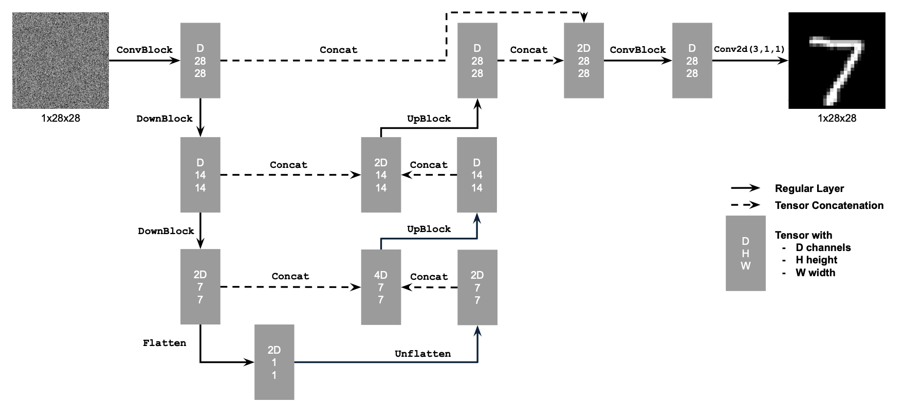
Figure 1: Unconditional UNet
The diagram above uses a number of standard tensor operations defined as follows:
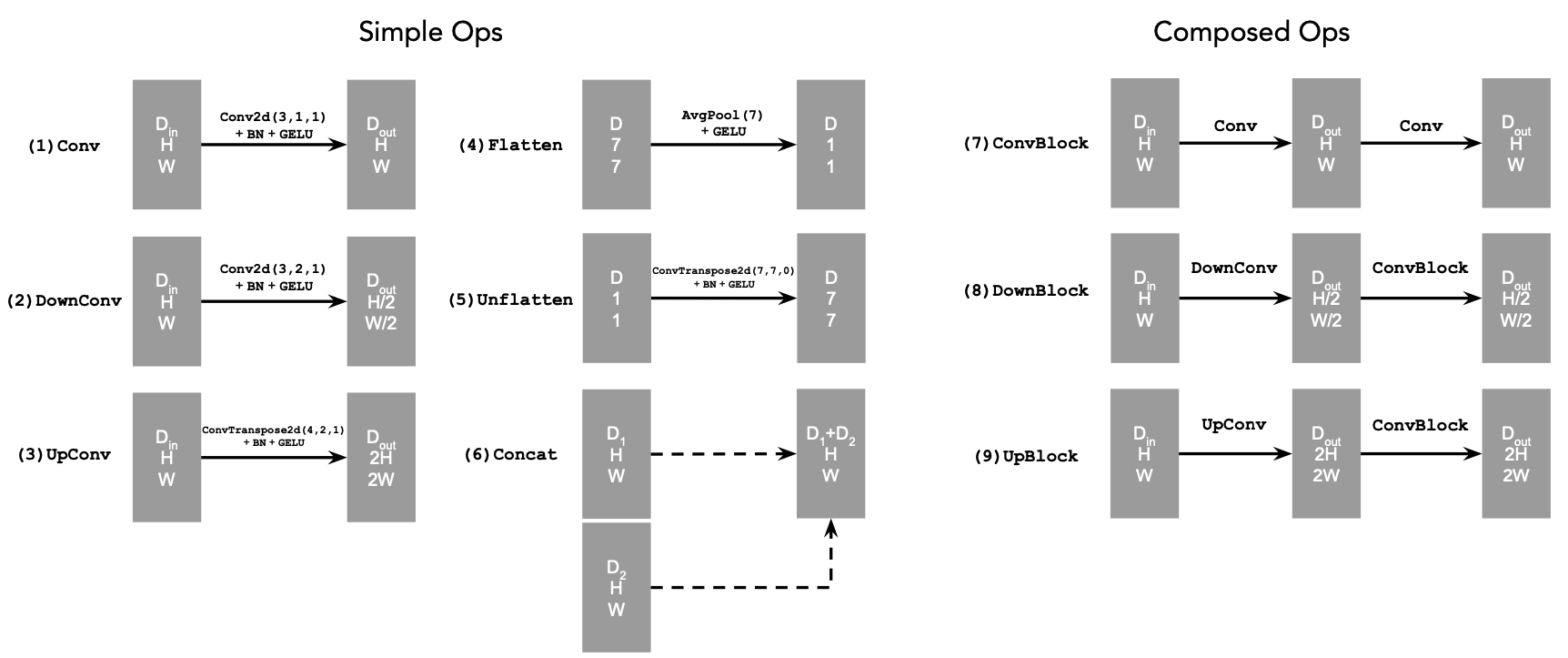
Figure 2: Standard UNet Operations
nn.Conv2d()nn.BatchNorm2d()nn.GELU()nn.ConvTranspose2d()nn.AvgPool2d()D is the number of hidden channels and is a
hyperparameter that we will set ourselves.torch.cat().We define composed operations using our simple operations in order to make our network deeper. This doesn't change the tensor's height, width, or number of channels, but simply adds more learnable parameters.
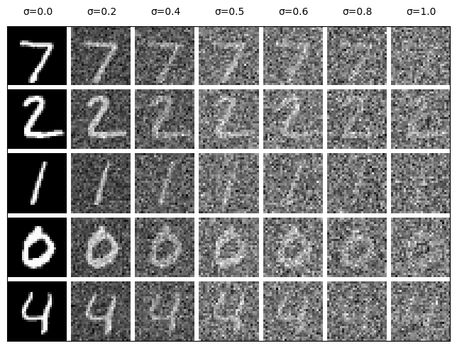
Figure 3: Varying levels of noise on MNIST digits
Now, we will train the model to perform denoising.
torchvision.datasets.MNIST with flags to access training
and test sets. Train only on the training set. Shuffle the dataset
before creating the dataloader. Recommended batch size: 256. We'll
train over our dataset for 5 epochs.
D = 128.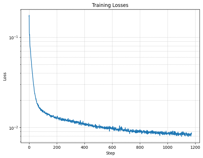
Figure 4: Training Loss Curve
They should look something like these:
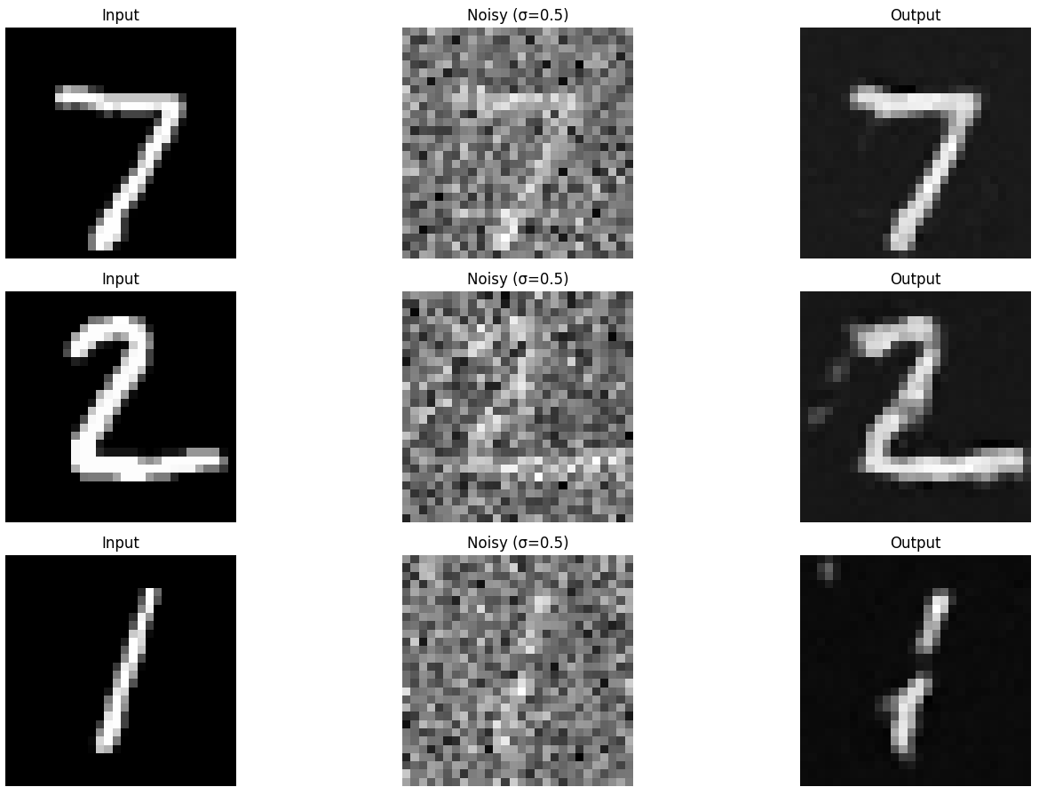
Figure 5: Results on digits from the test set after 1 epoch of training
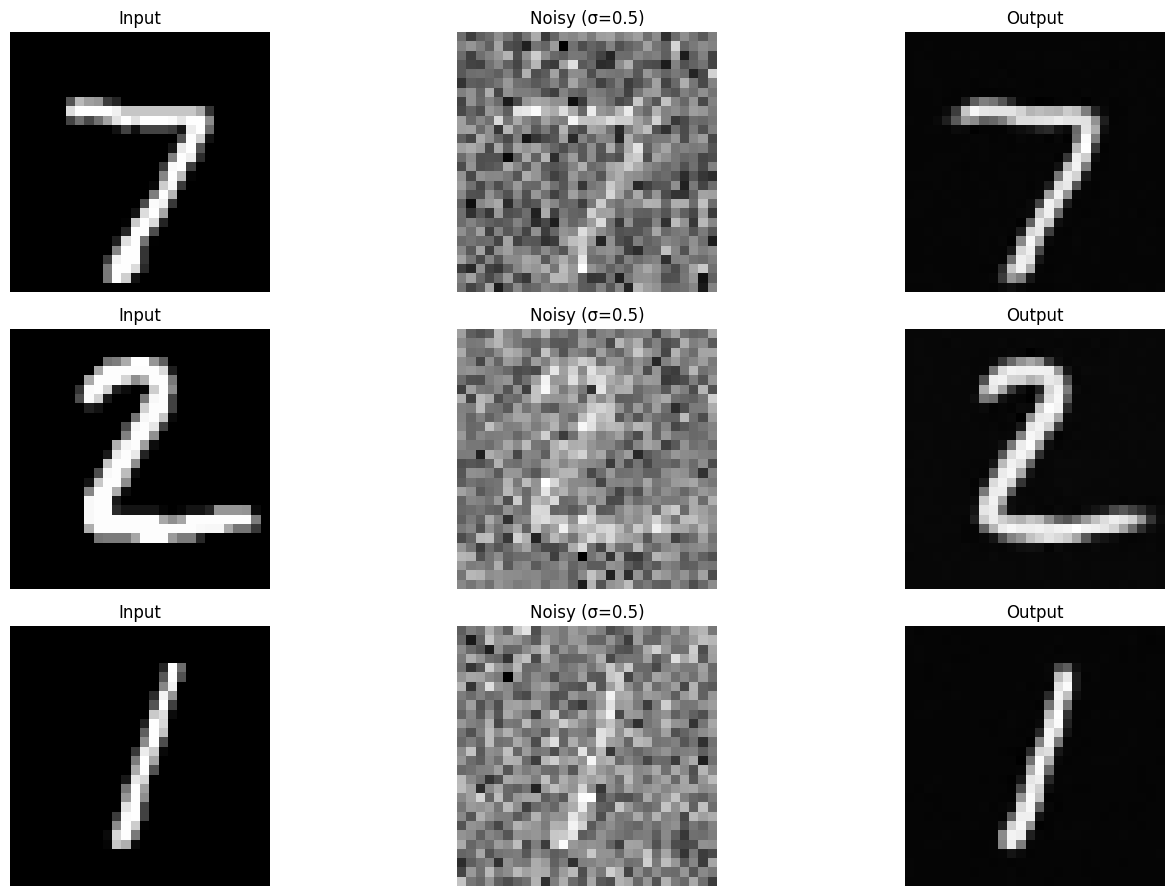
Figure 6: Results on digits from the test set after 5 epochs of training
Our denoiser was trained on MNIST digits noised with $\sigma = 0.5$. Let's see how the denoiser performs on different $\sigma$'s that it wasn't trained for.
Visualize the denoiser results on test set digits with varying levels of noise $\sigma = [0.0, 0.2, 0.4, 0.5, 0.6, 0.8, 1.0]$.
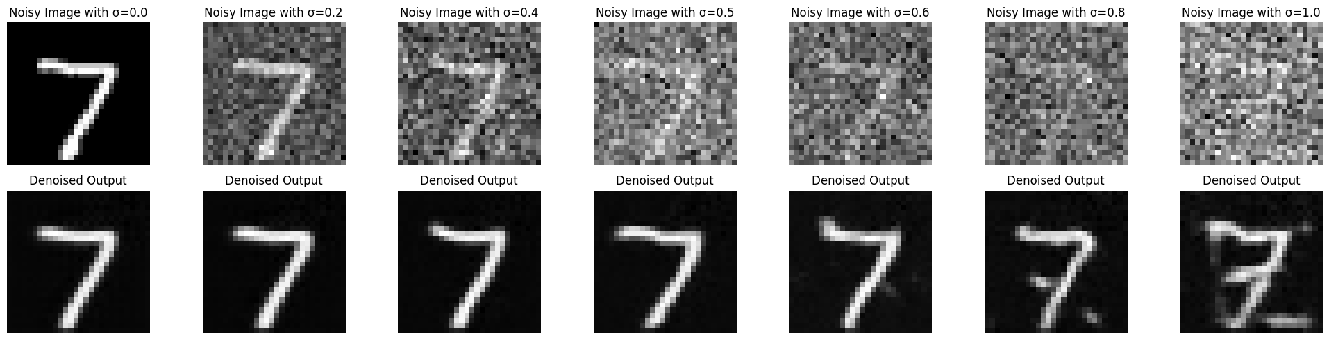
Figure 7: Results on digits from the test set with varying noise levels.
To make denoising a generative task, we'd like to be able to denoise pure, random Gaussian noise. We can think of this as starting with a blank canvas $z = \epsilon$ where $\epsilon \sim N(0, I)$ and denoising it to get a clean image $x$.
Repeat the same denoising process as in part 1.2.1, but start with pure noise $\epsilon \sim N(0, I)$ and denoise it for 5 epochs. Display your results after 1 and 5 epochs.
Additionally, compute the average image of the training set. What do you notice between the average image and our attempts to denoise pure noise? Why might this be happening?
We won't provide reference images for this part.
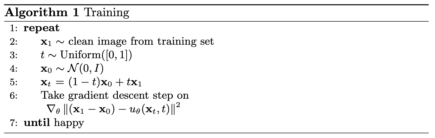
For iterative denoising, we need to define how intermediate noisy samples are constructed. The simplest approach would be a linear interpolation between noisy $x_0$ and clean $x_1$ for some $x_1$ in our training data:
\begin{equation} x_t = (1-t)x_0 + tx_1 \quad \text{where } x_0 \sim \mathcal{N}(0, 1), t \in [0, 1]. \tag{B.3} \end{equation} This is a vector field describing the position of a point $x_t$ at time $t$ relative to the clean data distribution $p_1(x_1)$ and the noisy data distribution $p_0(x_0)$. Intuitively, we see that for small $t$, we remain close to noise, while for larger $t$, we approach the clean distribution.Flow can be thought of as the velocity (change in posiiton w.r.t. time) of this vector field, describing how to move from $x_0$ to $x_1$: \begin{equation} u(x_t, t) = \frac{d}{dt} x_t = x_1 - x_0. \tag{B.4}\end{equation}
Our aim is to learn a UNet $u_\theta(x_t,t)$ which approximates this flow $u(x_t, t) = x_1 - x_0$, giving us our learning objective: \begin{equation} L = \mathbb{E}_{x_0 \sim p_0(x_0), x_1 \sim p_1(x_1), t \sim U[0, 1]} \|(x_1-x_0) - u_\theta(x_t, t)\|^2. \tag{B.5} \end{equation}
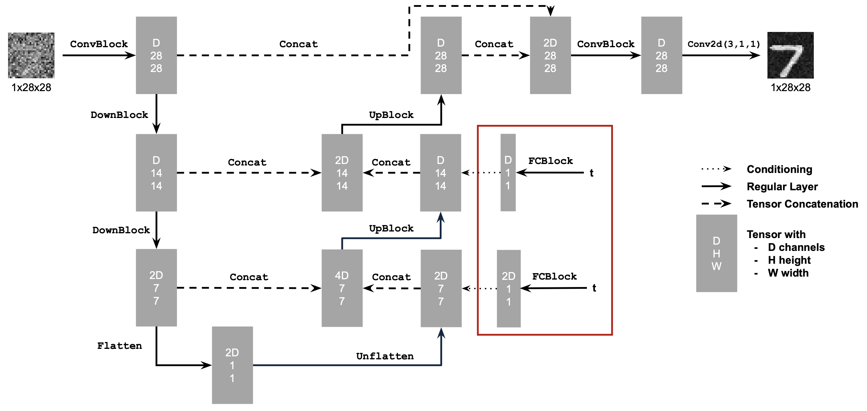
Figure 8: Conditioned UNet
Note: It may look like we're predicting the original image in the figure above, but we are not. We're predicting the flow from the noisy $x_0$ to clean $x_1$, which will contain both parts of the original image as well as the noise to remove.
This uses a new operator called FCBlock (fully-connected block) which we use to inject the conditioning signal into the UNet:
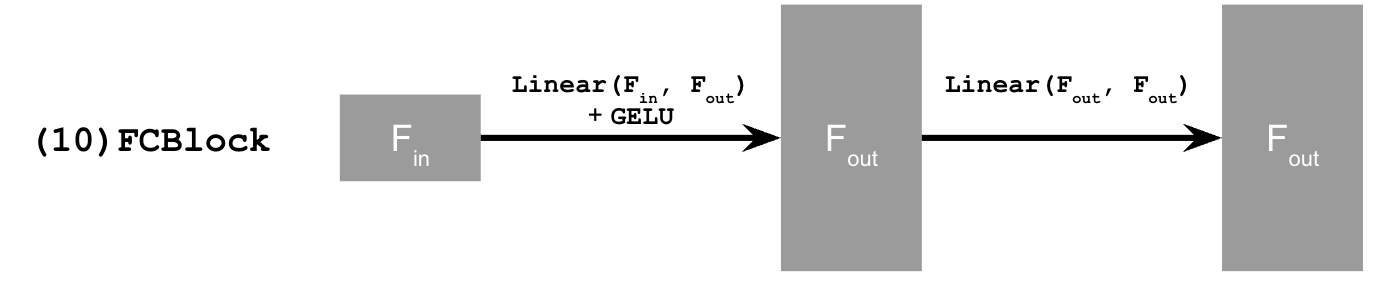
Figure 9: FCBlock for conditioning
nn.Linear.
Since our conditioning signal $t$ is a scalar, F_in should be of size 1.
You can embed $t$ by following this pseudo code:
fc1_t = FCBlock(...)
fc2_t = FCBlock(...)

# the t passed in here should be normalized to be in the range [0, 1]
t1 = fc1_t(t)
t2 = fc2_t(t)

# Follow diagram to get unflatten.
# Replace the original unflatten with modulated unflatten.
unflatten = unflatten * t1
# Follow diagram to get up1.
...
# Replace the original up1 with modulated up1.
up1 = up1 * t2
# Follow diagram to get the output.
...
Algorithm B.1. Training time-conditioned UNet
torchvision.datasets.MNIST with flags to access training
and test sets. Train only on the training set. Shuffle the dataset
before creating the dataloader. Recommended batch size: 64.
D = 64. Follow the diagram and pseudocode for how to inject the conditioning signal $t$ into the UNet. Remember to normalize $t$ before embedding it.scheduler = torch.optim.lr_scheduler.ExponentialLR(...). You should call scheduler.step() after every epoch.
Figure 10: Time-Conditioned UNet training loss curve
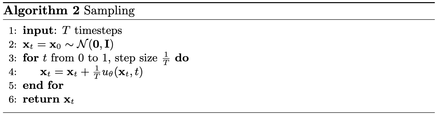
Algorithm B.2. Sampling from time-conditioned UNet
Epoch 1
Epoch 5
Epoch 10
Epoch 15
Epoch 20
fc1_t = FCBlock(...)
fc1_c = FCBlock(...)
fc2_t = FCBlock(...)
fc2_c = FCBlock(...)

t1 = fc1_t(t)
c1 = fc1_c(c)
t2 = fc2_t(t)
c2 = fc2_c(c)

# Follow diagram to get unflatten.
# Replace the original unflatten with modulated unflatten.
unflatten = c1 * unflatten + t1
# Follow diagram to get up1.
...
# Replace the original up1 with modulated up1.
up1 = c2 * up1 + t2
# Follow diagram to get the output.
...
Training for this section will be the same as time-only, with the only difference being the conditioning vector $c$ and doing unconditional generation periodically.
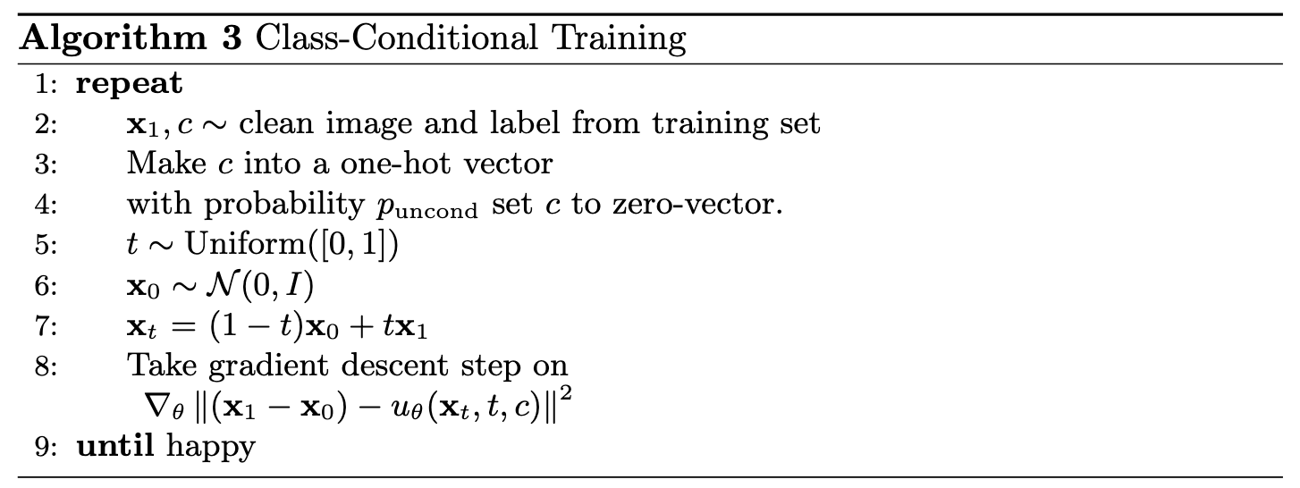
Algorithm B.3. Training class-conditioned UNet
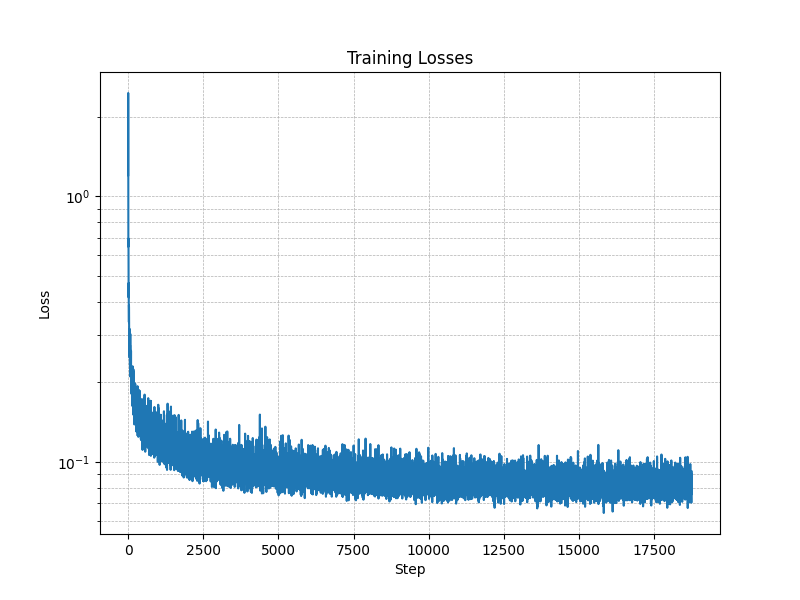
Figure 11: Class-conditioned UNet training loss curve
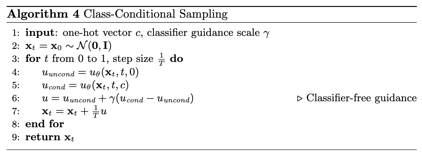
Algorithm B.4. Sampling from class-conditioned UNet
Epoch 1
Epoch 5
Epoch 10
Epoch 15
Epoch 20
This project originally had you implement DDPM instead of flow matching (flow matching can be thought of as a generalization of DDPM). If you'd like to implement DDPM, you can do so by following the original project instructions found here.
This project was a joint effort by Ryan Tabrizi, Daniel Geng, and Hang Gao, advised by Liyue Shen, Andrew Owens, Angjoo Kanazawa, and Alexei Efros. We also thank David McAllister and Songwei Yi for their helpful feedback and suggestions.