 Programming Project #5 (proj5)
CS180: Intro to Computer Vision and Computational Photography
Programming Project #5 (proj5)START EARLY!
This project, in many ways, will be the most difficult project this semester.Let's warmup by building a simple one-step denoiser. Given a noisy image $z$, we aim to train a denoiser $D_\theta$ such that it maps $z$ to a clean image $x$. To do so, we can optimize over an L2 loss: $$L = \mathbb{E}_{z,x} \|D_{\theta}(z) - x\|^2 \tag{1}$$
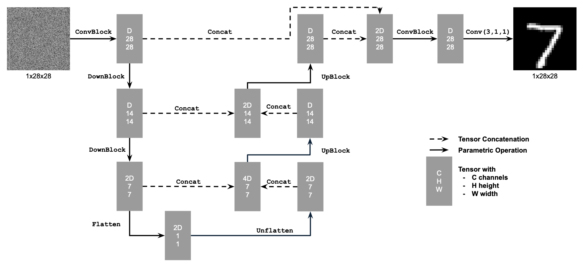
Figure 1: Unconditional UNet
The diagram above uses a number of standard tensor operations defined as follows:
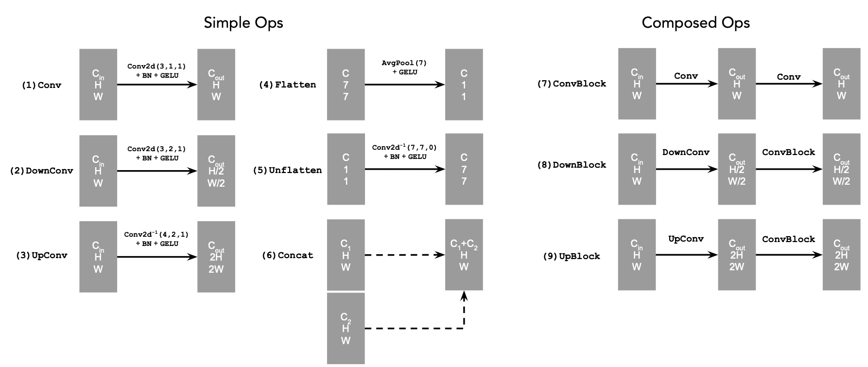
Figure 2: UNet Operations
torch.cat.D is the number of hidden channels and is a hyperparameter that we will set ourselves.We define composed operations using our simple operations in order to make our network deeper. This doesn't change the tensor's height, width, or number of channels, but simply adds more learnable parameters.
nn.Conv2d(kernel_size, stride, padding)nn.BatchNorm2dnn.GELU()nn.ConvTranspose2d(kernel_size, stride, padding)nn.AvgPool2d(kernel_size)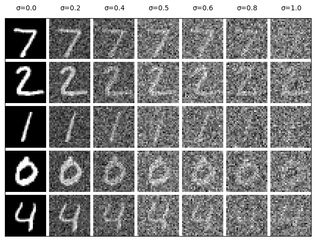
Figure 3. Varying levels of noise on MNIST digits
Now, we will train the model to perform denoising.
torchvision.datasets.MNIST with flags to access training and test sets. Shuffle the dataset before creating the dataloader. Recommended batch size: 256. We'll train over our dataset for 5 epochs.
D in the diagrams above).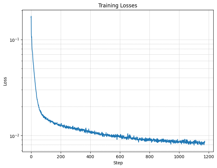
Figure 4. Training Loss Curve
They should look something like these:
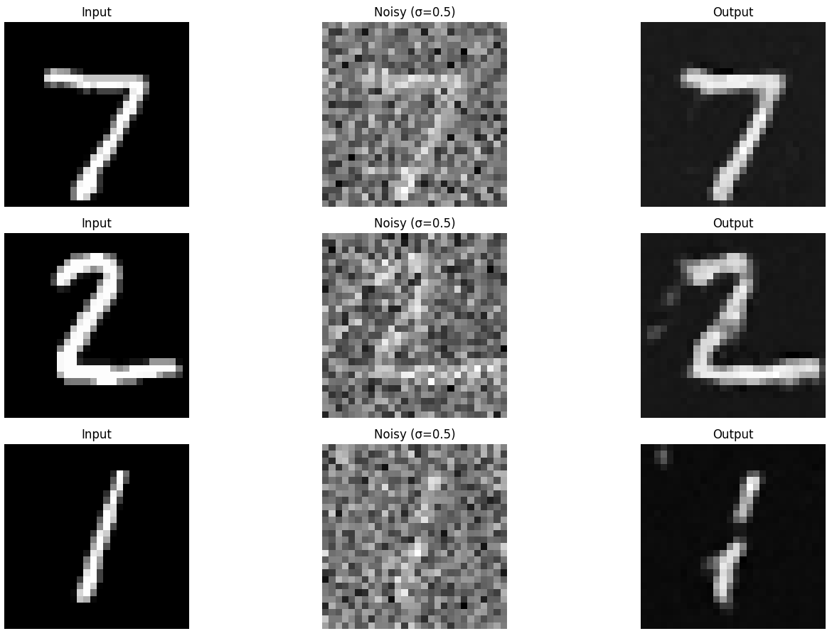
Figure 5. Results on digits from the test set after 1 epoch of training
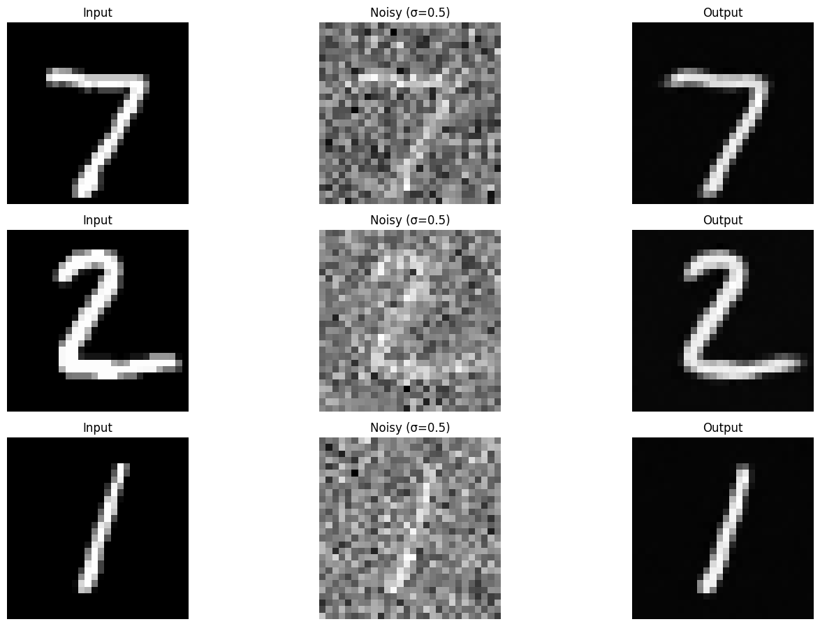
Figure 6. Results on digits from the test set after 5 epochs of training
Our denoiser was trained on MNIST digits noised with $\sigma = 0.5$. Let's see how the denoiser performs on different $\sigma$'s that it wasn't trained for.
Visualize the denoiser results on test set digits with varying levels of noise $\sigma = [0.0, 0.2, 0.4, 0.5, 0.6, 0.8, 1.0]$.
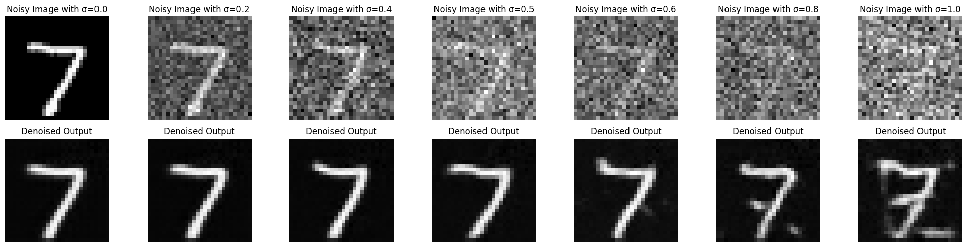
Figure 7. Results on digits from the test set with varying noise levels.
One small change is that we're going to change our UNet from part 1 to predict the noise instead of the clean image (like in part 4A of the project).
Let's reconsider the problem in part 1, but to its extreme:
Given a pure noise image $\epsilon \sim N(0, I)$, we aim to train a denoiser $D_{\theta}$ such that it maps the noise image to a clean image $x$. To do so, we can still apply a simple L2 loss:
$$L = \mathbb{E}_{\epsilon,x} \|D_{\theta}(\epsilon) - x\|^2.$$
The difference here, compared to part 1, is that $\epsilon$ is pure noise. If we can learn to remove pure noise, this will allow us to generate novel images, not just those in our training set.
However, we saw in part A that one-step denoising does not yield good results. Instead, we can iteratively denoise the image for better results.
For iterative denoising, we condition our model on timestep $t$ such that it can learn time-specific denoising. We can equivalently predict the noise added to the image rather than the denoised image itself.
$$L = \mathbb{E}_{\epsilon,x_0,t} \|\epsilon_{\theta}(x_t, t) - \epsilon\|^2. \tag{3}$$
$$\text{where }x_t = a_t x_0 + b_t \epsilon,~x_T := \epsilon$$ $$~t \in \{0, 1, \cdots, T\},~\epsilon \sim N(0, I).$$
For now, $a_t$ and $b_t$ can be thought of as some random function of $t$.
You can imagine that, with a time-conditioned denoising UNet, we can go from one-step denoising to iterative denoising:
$$x_{T-1} = x_T - \epsilon_\theta(x_T; T)$$ $$x_{T-2} = x_{T-1} - \epsilon_\theta(x_{T-1}; T-1)$$ $$\cdots$$ $$x_0 = x_{1} - \epsilon_\theta(x_{1}; 1).$$
We can therefore perform iterative denoising to get better results than a one-step denoiser as shown in part 1, which is especially useful when our noisy inputs are pure Gaussian noise.
In practice, our model is predicting the entire noise added to $x_0$ to get $x_t$ rather than intermediate amounts of noise, but the coefficients $a_t$ and $b_t$ will appropriately scale such that we recover intermediate noise samples $x_i$ for $i \in \{1, \cdots, T-1\}$. Additionally, because of this scaling we cannot directly subtract the noise as shown above, but will instead do so under a different process shown later.
Let's first define a new operator called FCBlock (fully-connected block):
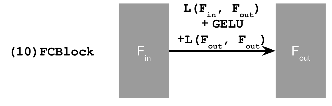
Figure 8. FCBlock for conditioning
nn.Linear.
To condition our network on time and class-label, we can apply conditioning after unflattening and the first upsample:
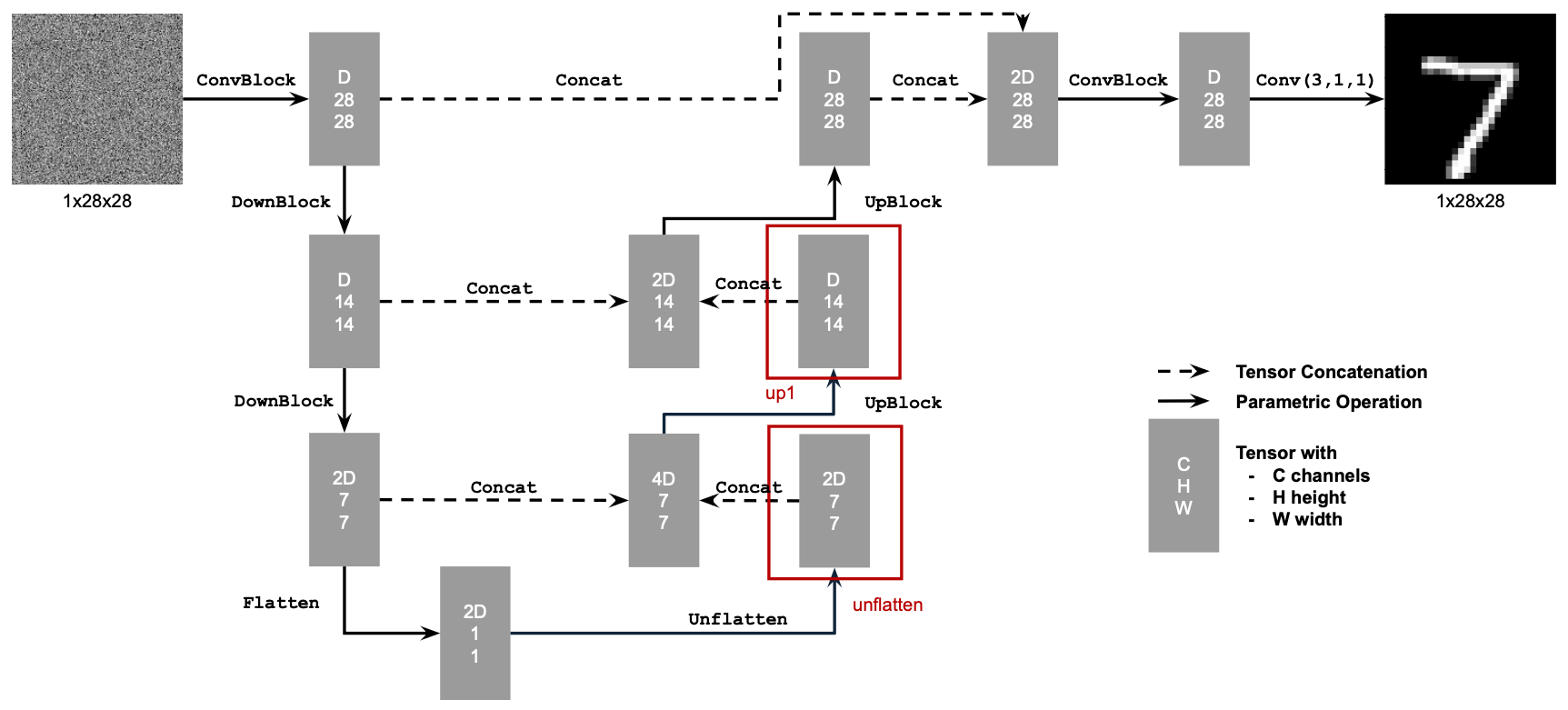
Figure 9. Conditional UNet
You can embed $t$ and $c$ by following this pseudo code:
fc1_t = FCBlock(...)
fc1_c = FCBlock(...)
fc2_t = FCBlock(...)
fc2_c = FCBlock(...)

t1 = fc1_t(t)
c1 = fc1_c(c)
t2 = fc2_t(t)
c2 = fc2_c(c)

# Follow diagram to get unflatten.
# Replace the original unflatten with modulated unflatten.
unflatten = fc1_c * unflatten + fc1_t
# Follow diagram to get up1.
...
# Replace the original up1 with modulated up1.
up1 = fc2_c * up1 + fc2_t
# Follow diagram to get the output.
...
Note that the class-label $c$ should be encoded as one-hot vector.
Another modification you need to make is to make model take in a batch-wise mask vector which is either 0 or 1. It indicates whether or not to drop the condition $c$: drop when mask is 0, not drop when mask is 1. It can be null, which means just using the condition. This is so we can perform line 6 of algorithm 1.
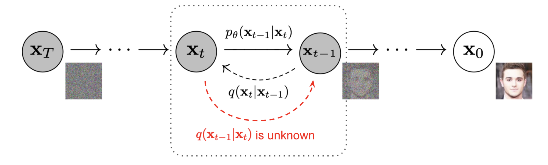
Figure 10: DDPM markov chain. The forward process is
denoted by $q(x_t\mid x_{t-1})$ and the reverse process is denoted
by $p_\theta(x_{t-1}\mid x_t)$.
(Image source: Ho et al. 2020 with a few additional annotations
from Lilian Weng)
Specifically, each forward step adds Gaussian noise in a variance-preserving way for some variance schedule $\{\beta_t\}_{t=1}^T$:
Using the reparamaterization trick presented in section 2 of the DDPM paper, we can compute effective one step noising function, since a Gaussian convolved with a Gaussian is still Gaussian (see here for more details).
Concretely, let $\alpha_t := 1 -\beta_t$ and $\bar{\alpha_t} := \prod^t_{s=1}\alpha_s$, then we can sample a noisy $x_t$ for an arbitrary $t$:
Let's first implement the DDPM scheduler to fetch all relevant variables. Given $(\beta_0, \beta_T, T)$, follow the doc-string to get all useful values. You will use them in a bit!
TODO: Implementddpm_schedule()
For brevity, we don't show the mathematical details here. If you'd like to see the mathematical details, check out here.
TODO: Implement ourddpm_forward() function by
following algorithm 1:
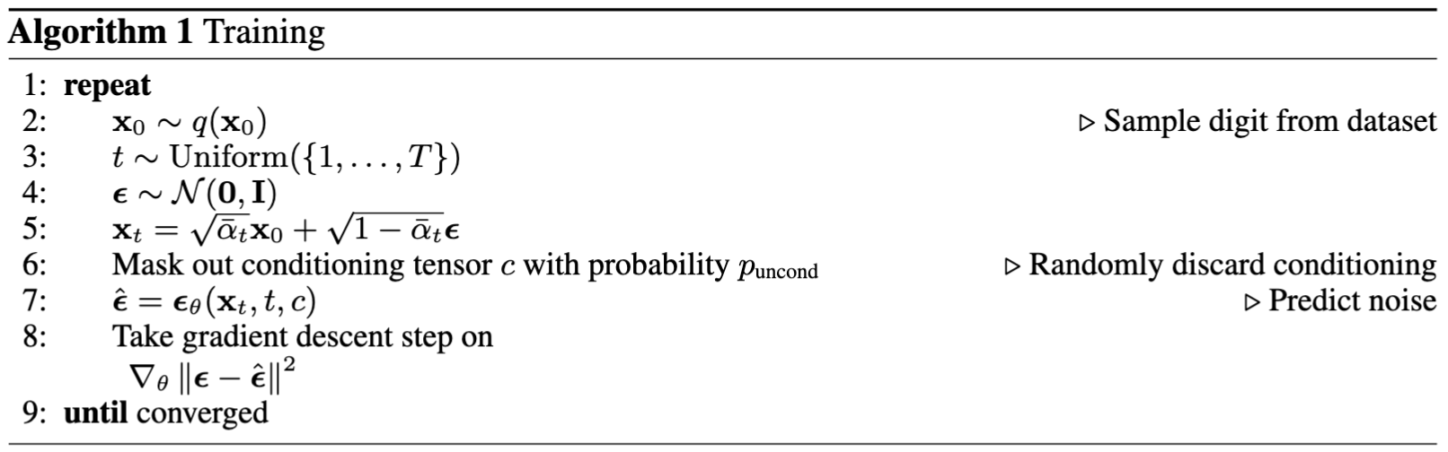
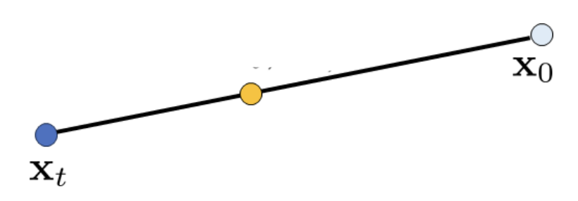
Figure 11: Interpolation of $x_0$ and $x_t$
(Image source)
Using the same reparamaterization trick from equation 5, we can solve for $x_0$: $$x_0 = \frac{1}{\sqrt{\bar{\alpha}_t}} \left( \mathbf{x}_t - \sqrt{1 - \bar{\alpha}_t} \epsilon_t \right),\tag{8}$$
If we plug this back into equation 7, we get: $$\tilde{\mu}_(\mathbf{x}_t, x_0) := \frac{1}{\sqrt{\alpha_t}}(\mathbf{x}_t - \frac{1 - \alpha_t}{\sqrt{1 - \bar{\alpha}_t}}\epsilon_t)\tag{9}$$
Thus, by using the reparameterization trick and following equation 6, we can cleanly represent $x_{t-1}$ as: $$\mathbf{x}_{t-1} = \tilde{\mu}_t(\mathbf{x}_t, \mathbf{x}_0) + \sqrt{\tilde{\beta}_t} \mathbf{z}, \quad \mathbf{z} \sim \mathcal{N}(0, \mathbf{I})\tag{10}$$ $$\implies \mathbf{x}_{t-1} = \frac{1}{\sqrt{\alpha_t}}(\mathbf{x}_t - \frac{1 - \alpha_t}{\sqrt{1 - \bar{\alpha}_t}}\epsilon_t) + \sigma_t \mathbf{z}, \quad \text{where } \sigma_t = \sqrt{\tilde{\beta}_t}\tag{11}$$To model this, we train network $\mu_\theta(x_t, x_0)$ We don't need to learn the $\sigma_t$ term (since it is defined by the schedule), therefore we only optimize $\mu_\theta(x_t, x_0)$.
Similarly, we have access to $\mathbf{x}_t$ and $\alpha$ terms, so we only need to optimize a network $\epsilon_\theta(x_t, t)$ to predict the noise term.
TODO: Implement the reverse sampling processddpm_sample():
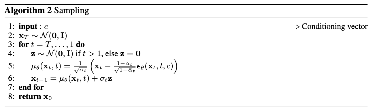
Again, if you are interested in the math, check out here.
Some important details:
seed, then shift your
seed by 1 each denoising step.unet twice, one with mask =
torch.ones(...) and one with mask =
torch.zeros(...). You could do it in one batch, but it
is easy to make mistake. So I would suggest to just forward it
twice.caches. It is just the
cache for some intermediate sampling results for animation. How
to cache this is your choice, but we suggest the following
way:if t[0] % 20 == 0 or t[0] == num_ts or t[0] < 8:
caches.append(x)
We have all the pieces, let's now train our diffusion model. Please consider this pseudo code for your training step.
def train_step():
    x0 = sample_from_data()

    t = uniform_sample_T()
    loss = diffusion_forward(x0, t)

    optimizer.zero_grad()
    loss.backward()
    optimizer.step()
Use the same network hyperparameters as in part 1.
You might need to increase num_epochs = 20 to get
good results (staff solution takes ~26 minutes on a Colab T4 GPU)
Your deliverables should include the following for this problem:
guidance_scale = 5.guidance_scale = [0, 5, 10].Epoch 1
Epoch 5
Epoch 10
Epoch 15
Epoch 20
This project was a joint effort by Daniel Geng, Hang Gao, and Ryan Tabrizi, advised by Liyue Shen, Andrew Owens, and Alexei Efros.