Instead of asking ChatGPT to write everything for you, please consult the following resources when you get stuck —
they will help you understand how and why things work under the hood.
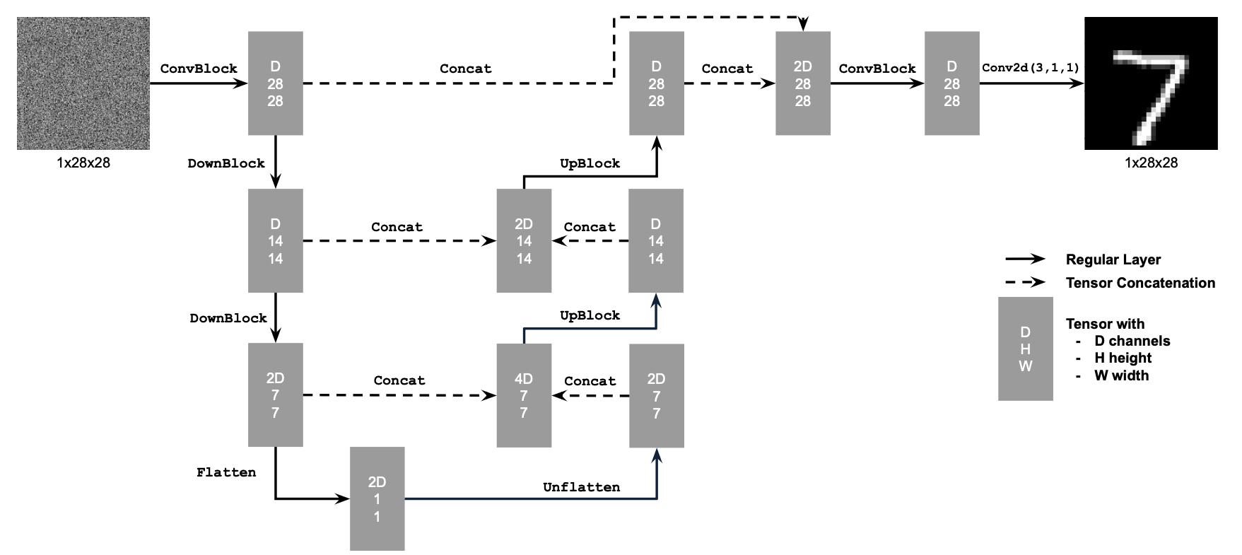
Let's warmup by building a simple one-step denoiser. Given a noisy image
$z$, we
aim to train a denoiser $D_\theta$ such that it maps $z$ to a clean
image $x$. To do so, we can optimize over an L2 loss:
$$L = \mathbb{E}_{z,x} \|D_{\theta}(z) - x\|^2 \tag{B.1}$$
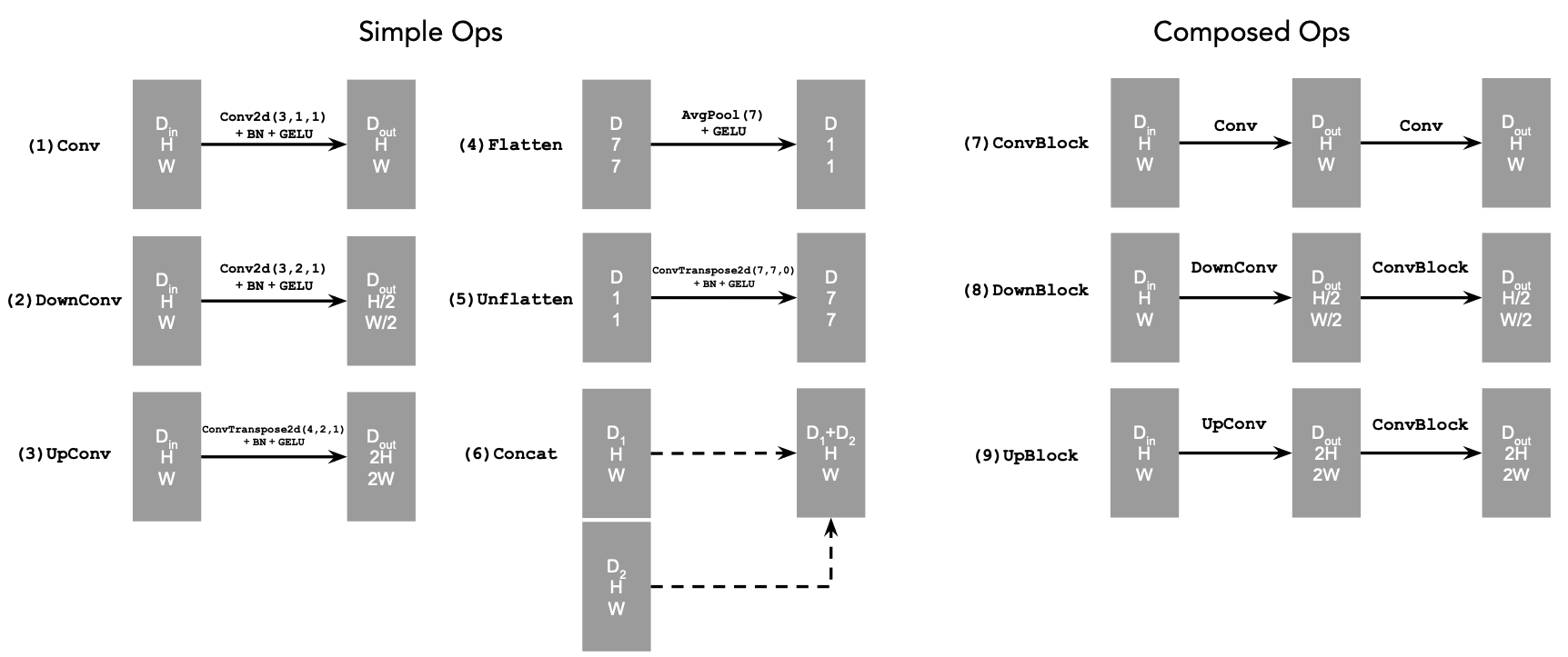
The diagram above uses a number of standard tensor operations defined as
follows:
where:
- Conv2d(kernel_size, stride, padding) is
nn.Conv2d()
- BN is
nn.BatchNorm2d()
- GELU is
nn.GELU()
- ConvTranspose2d(kernel_size, stride, padding) is
nn.ConvTranspose2d()
- AvgPool(kernel_size) is
nn.AvgPool2d()
D is the number of hidden channels and is a
hyperparameter that we will set ourselves.
At a high level, the blocks do the following:
- (1) Conv is a convolutional layer that doesn't
change the image resolution, only the channel dimension.
- (2) DownConv is a convolutional layer that
downsamples the tensor by 2.
- (3) UpConv is a convolutional layer that upsamples
the tensor by 2.
- (4) Flatten is an average pooling layer that
flattens a 7x7 tensor into a 1x1 tensor. 7 is the resulting height and
width after the downsampling operations.
- (5) Unflatten is a convolutional layer that
unflattens/upsamples a 1x1 tensor into a 7x7 tensor.
- (6) Concat is a channel-wise concatenation between
tensors with the same 2D shape. This is simply
torch.cat().
We define composed operations using our simple operations in order to
make our network deeper. This doesn't change the tensor's height, width,
or number of channels, but simply adds more learnable parameters.
1.2 Using the UNet to Train a Denoiser
Recall from equation 1 that we aim to solve the following denoising
problem:
Given a noisy image $z$, we
aim to train a denoiser $D_\theta$ such that it maps $z$ to a clean
image $x$. To do so, we can optimize over an L2 loss
$$
L = \mathbb{E}_{z,x} \|D_{\theta}(z) - x\|^2.
$$
To train our denoiser, we need to generate training data pairs of ($z$,
$x$), where each $x$ is a clean MNIST digit. For each training batch, we
can generate $z$ from $x$ using the the following noising process:
$$
z = x + \sigma \epsilon,\quad \text{where }\epsilon \sim N(0, I). \tag{B.2}
$$
Visualize the different noising processes over $\sigma = [0.0, 0.2, 0.4,
0.5, 0.6, 0.8, 1.0]$, assuming normalized $x \in [0, 1]$.
You should see noisier images as $\sigma$ increases.
Deliverable
- A visualization of the noising process using $\sigma = [0.0,
0.2, 0.4, 0.5, 0.6, 0.8, 1.0]$.
1.2.1 Training
Now, we will train the model to perform denoising.
- Objective: Train a denoiser to denoise noisy image $z$ with
$\sigma = 0.5$ applied to a clean image $x$.
- Dataset and dataloader: Use the MNIST dataset via
torchvision.datasets.MNIST。 Train only on the training set.
Shuffle the dataset before creating the dataloader. Recommended batch
size: 256. We'll train over our dataset for 5 epochs.
- You should only noise the image batches when fetched from the
dataloader so that in every epoch the network will see new noised
images due to a random $\epsilon$, improving generalization.
- Model: Use the UNet architecture defined in section 1.1 with
recommended hidden dimension
D = 128.
- Optimizer: Use Adam optimizer with learning rate of
1e-4.
You should visualize denoised results on the test set at the end of
training. Display sample results after the 1st and 5th epoch.
After 5 epoch training, they should look something like these:
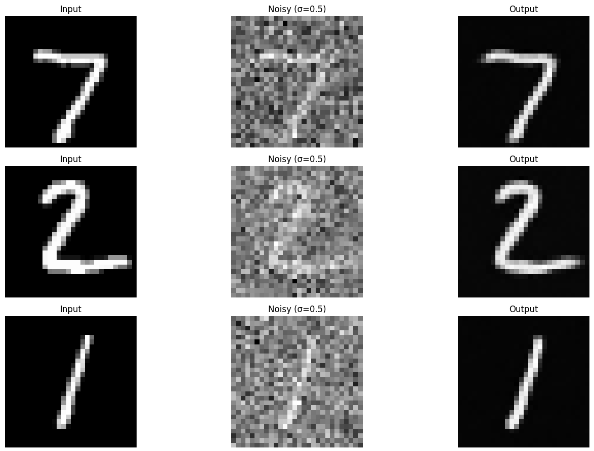
Figure 3: Results on digits from the test set after 5
epochs of training
Deliverables
- A training loss curve plot every few iterations during the whole
training process of $\sigma = 0.5$.
- Sample results on the test set with noise level 0.5 after the first and the 5-th epoch
(staff solution takes ~3 minutes for 5 epochs on a Colab T4 GPU).
1.2.2 Out-of-Distribution Testing
Our denoiser was trained on MNIST digits noised with $\sigma = 0.5$. Let's
see how the denoiser performs on different $\sigma$'s that it wasn't
trained for.
Visualize the denoiser results on test set digits with varying levels of
noise $\sigma = [0.0, 0.2, 0.4, 0.5, 0.6, 0.8, 1.0]$.
Deliverables
- Sample results on the test set with out-of-distribution noise levels
after the model is trained. Keep the same image and
vary $\sigma = [0.0, 0.2, 0.4, 0.5, 0.6, 0.8, 1.0]$.
1.2.3 Denoising Pure Noise
To make denoising a generative task, we'd like to be able to denoise pure, random Gaussian noise. We can think of this as starting with a blank canvas $z = \epsilon$ where $\epsilon \sim N(0, I)$ and denoising it to get a clean image $x$.
Repeat the same training process as in part 1.2.1, but input pure noise $\epsilon \sim N(0, I)$ and denoise it for 5 epochs. Display your results after 1 and 5 epochs.
Sample from the denoiser that was trained to denoise pure noise. What patterns do you observe in the generated outputs? What relationship, if any, do these outputs have with the training images (e.g., digits 0–9)? Why might this be happening?
Deliverables
- A training loss curve plot every few iterations during the whole
training process that denoises pure noise.
- Sample results on pure noise after the first and the 5-th epoch.
- A brief description of the patterns observed in the generated outputs and explanations for why they may exist.
Hint
-
For the last question, recall that with an MSE loss, the model learns to predict the point that
minimizes the sum of squared distances to all training examples. This is
closely related to the idea of a centroid in clustering. What does it
represent in the context of the training images?
- Since training can take a while, we strongly recommend that you
checkpoint your model every epoch onto your personal Google
Drive.
This is because Colab notebooks aren't persistent such that if you are
idle for a while, you will lose connection and your training progress.
This consists of:
- Google Drive mounting.
- Epoch-wise model & optimizer checkpointing.
- Model & optimizer resuming from checkpoints.
Part 2: Training a Flow Matching Model
We just saw that one-step denoising does not work well for generative tasks. Instead, we need to iteratively denoise the image, and we will do so with flow matching.
Here, we will iteratively denoise an image by training a UNet model to predict the `flow' from our noisy data to clean data.
In our flow matching setup, we sample a pure noise image $x_0 \sim \mathcal{N}(0, I)$ and generate a realistic image $x_1$.
For iterative denoising, we need to define how intermediate noisy samples are constructed. The simplest approach would be a linear interpolation between noisy $x_0$ and clean $x_1$ for some $x_1$ in our training data:
\begin{equation}
x_t = (1-t)x_0 + tx_1 \quad \text{where } x_0 \sim \mathcal{N}(0, 1), t \in [0, 1]. \tag{B.3}
\end{equation}
This is a vector field describing the position of a point $x_t$ at time $t$ relative to the clean data distribution $p_1(x_1)$ and the noisy data distribution $p_0(x_0)$. Intuitively, we see that for small $t$, we remain close to noise, while for larger $t$, we approach the clean distribution.
Flow can be thought of as the velocity (change in posiiton w.r.t. time) of this vector field, describing how to move from $x_0$ to $x_1$:
\begin{equation} u(x_t, t) = \frac{d}{dt} x_t = x_1 - x_0. \tag{B.4}\end{equation}
Our aim is to learn a UNet $u_\theta(x_t,t)$ which approximates this flow $u(x_t, t) = x_1 - x_0$, giving us our learning objective:
\begin{equation}
L = \mathbb{E}_{x_0 \sim p_0(x_0), x_1 \sim p_1(x_1), t \sim U[0, 1]} \|(x_1-x_0) - u_\theta(x_t, t)\|^2. \tag{B.5}
\end{equation}
2.1 Adding Time Conditioning to UNet
We need a way to inject scalar $t$ into our UNet model to condition it. There are many ways to do this. Here is what we suggest:
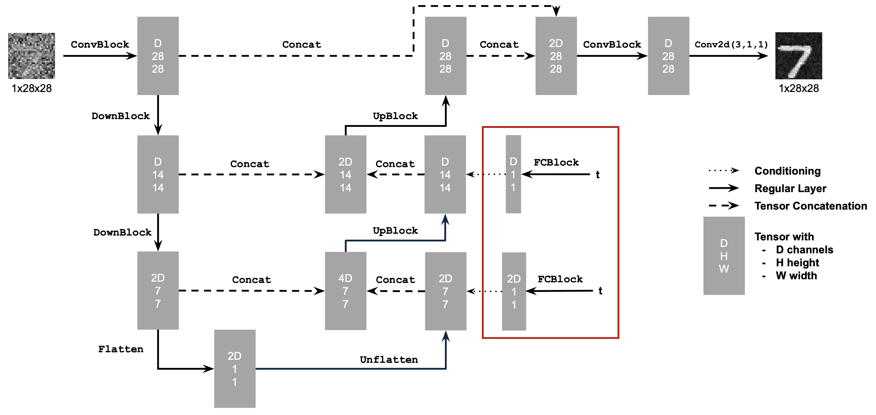
Figure 4: Conditioned UNet
Note: It may look like we're predicting the original image in the figure above, but we are not. We're predicting the flow from the noisy $x_0$ to clean $x_1$, which will contain both parts of the original image as well as the noise to remove.
This uses a new operator called
FCBlock (fully-connected block) which we use to inject the conditioning signal into the UNet:
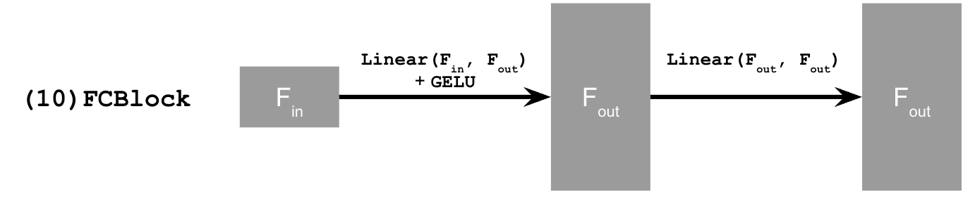
Figure 5: FCBlock for conditioning
Here Linear(F_in, F_out) is a linear layer with
F_in input features and F_out output
features. You can implement it using nn.Linear.
Since our conditioning signal $t$ is a scalar, F_in should be of size 1.
You can embed $t$ by following this pseudo code:
fc1_t = FCBlock(...)
fc2_t = FCBlock(...)

# the t passed in here should be normalized to be in the range [0, 1]
t1 = fc1_t(t)
t2 = fc2_t(t)

# Follow diagram to get unflatten.
# Replace the original unflatten with modulated unflatten.
unflatten = unflatten * t1
# Follow diagram to get up1.
...
# Replace the original up1 with modulated up1.
up1 = up1 * t2
# Follow diagram to get the output.
...
2.2 Training the UNet
Training our time-conditioned UNet $u_\theta(x_t, t)$ is now pretty easy. Basically, we pick a random image $x_1$
from the training set, a random timestep $t$, add noise to $x_1$ to get $x_t$, and train the denoiser to predict the flow at $x_t$. We repeat this for different images and different timesteps until the model converges and we are happy.
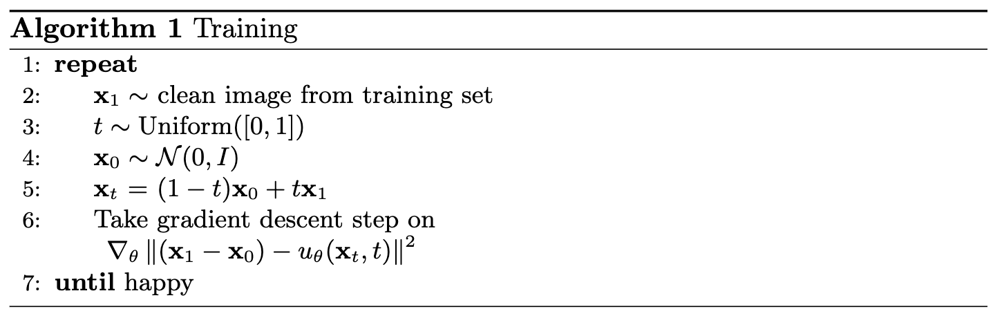
Algorithm B.1. Training time-conditioned UNet
- Objective: Train a time-conditioned UNet $u_\theta(x_t, t)$ to predict the flow at $x_t$ given a noisy image $x_t$ and a timestep $t$.
- Dataset and dataloader: Use the MNIST dataset via
torchvision.datasets.MNIST. Train only on the training set. Shuffle the dataset
before creating the dataloader. Recommended batch size: 64.
- As shown in algorithm B.1, You should only noise the image batches when fetched from the
dataloader.
- Model: Use the time-conditioned UNet architecture defined in section 2.1 with
recommended hidden dimension
D = 64. Follow the diagram and pseudocode for how to inject the conditioning signal $t$ into the UNet. Remember to normalize $t$ before embedding it.
- Optimizer: Use Adam optimizer with an initial learning rate of
1e-2. We will be using an exponential learning rate decay scheduler with a gamma of $0.1^{(1.0 / \text{num_epochs})}$. This can be implemented using
scheduler = torch.optim.lr_scheduler.ExponentialLR(...). You should call scheduler.step() after every epoch.
Deliverable
- A training loss curve plot for the time-conditioned UNet over the whole training process.
2.3 Sampling from the UNet
We can now use our UNet for iterative denoising using the algorithm below! The results would not be perfect, but legible digits should emerge
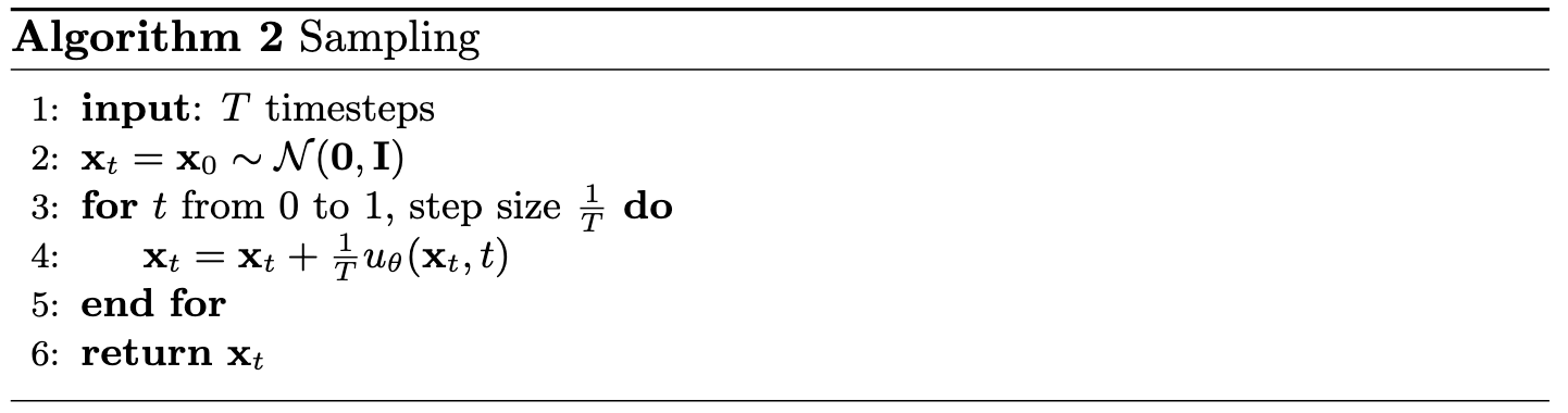
Algorithm B.2. Sampling from time-conditioned UNet
Deliverables
- Sampling results from the time-conditioned UNet for 1, 5, and 10 epochs. The results should not be perfect, but reasonably good.
- (Optional for CS180, required for CS280A) Check the Bells and Whistles if you want to make it better!
2.4 Adding Class-Conditioning to UNet
To make the results better and give us more control for image generation, we can also optionally condition our UNet on the class of the digit 0-9. This will require adding 2 more FCBlocks to our UNet but, we suggest that for class-conditioning vector $c$, you make it a one-hot vector instead of a single scalar.
Because we still want our UNet to work without it being conditioned on the class (recall the classifer-free guidance you implemented in part a), we implement dropout where 10% of the time ($p_{\text{uncond}}= 0.1$) we drop the class conditioning vector $c$ by setting it to 0.
Here is one way to condition our UNet $u_\theta(x_t, t, c)$ on both time $t$ and class $c$:
fc1_t = FCBlock(...)
fc1_c = FCBlock(...)
fc2_t = FCBlock(...)
fc2_c = FCBlock(...)

t1 = fc1_t(t)
c1 = fc1_c(c)
t2 = fc2_t(t)
c2 = fc2_c(c)

# Follow diagram to get unflatten.
# Replace the original unflatten with modulated unflatten.
unflatten = c1 * unflatten + t1
# Follow diagram to get up1.
...
# Replace the original up1 with modulated up1.
up1 = c2 * up1 + t2
# Follow diagram to get the output.
...
2.5 Training the UNet
Training for this section will be the same as time-only, with the only difference being the conditioning vector $c$ and doing unconditional generation periodically.
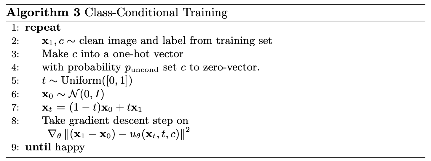
Algorithm B.3. Training class-conditioned UNet
Deliverable
- A training loss curve plot for the class-conditioned UNet over the whole training process.
2.6 Sampling from the UNet
Now we will sample with class-conditioning and will use classifier-free guidance with $\gamma = 5.0$.
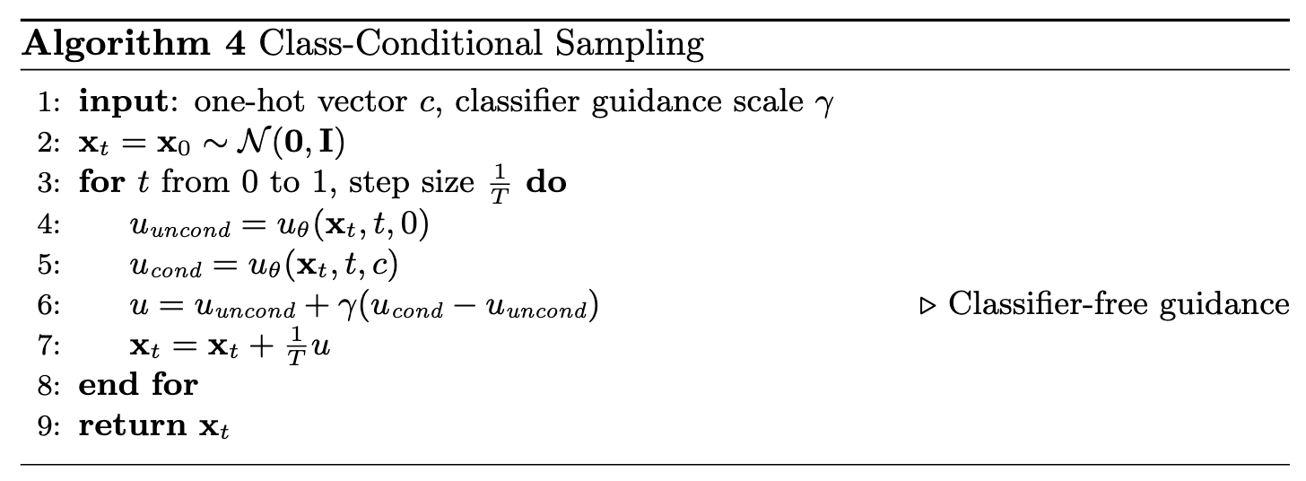
Algorithm B.4. Sampling from class-conditioned UNet
Deliverables
- Sampling results from the class-conditioned UNet for 1, 5, and 10 epochs. Class-conditioning lets us converge faster, hence why we only train for 10 epochs. Generate 4 instances of each digit as shown above.
- Can we get rid of the annoying learning rate scheduler? Simplicity is the best. Please try to maintain the same performance after removing the exponential
learning rate scheduler. Show your visualization after training without the scheduler and provide a description of what you did to compensate for the loss of the scheduler.
Part 3: Bells & Whistles
Required for CS280A students only:
- A better time-conditioned only UNet: Our time-conditioning only UNet in part 2.3 is actually far from perfect. Its result is way worse than the UNet conditioned by both time and class.
We can definitively make it better! Show a better visualization image for the time-conditioning only network. Possible approaches include extending the training schedule or making the architecture more expressive.
Optional for all students:
- Your own ideas: Be creative! This UNet can generate images more than digits! You can try it on SVHN (still digits, but more fancy!), Fashion-MNIST (not digits, but still grayscale!), or CIFAR10!
Deliverable Checklist
- Make sure that your website and submission include all the deliverables in each section above.
- Submit your PDF and code to corresponding assignments on Gradescope.
-
The Google Form is required for Part B. Once you have finished both parts A and B, submit the link to your webpage (containing both parts) using this
Google Form.
Acknowledgements
This project was a joint effort by Ryan Tabrizi, Daniel Geng, Hang Gao, and Jingfeng Yang, advised by Liyue Shen, Andrew Owens,
Angjoo Kanazawa,
and Alexei
Efros. We also thank David McAllister and Songwei Ge for their helpful feedback and suggestions.
 Programming Project #5 (