Programming Project #3 (proj3)
CS180: Intro to Computer Vision and Computational Photography
University of California, Berkeley

Text-Guided Editing

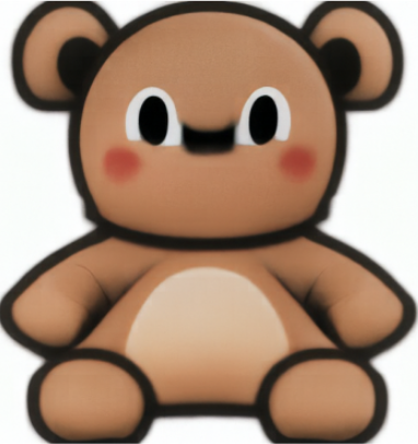
"Make it Real"

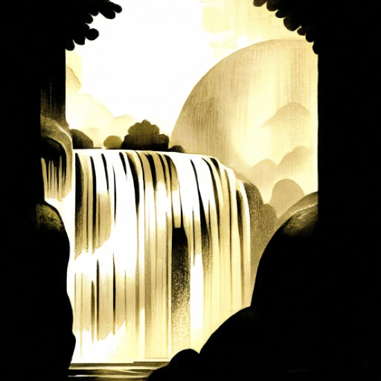
Waterfall / Skull Hybrid

A Lithograph of a Skull

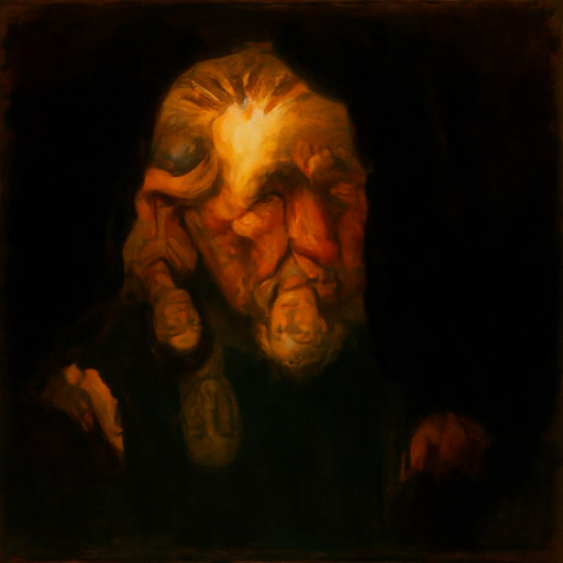
Old Man / Campfire Anagram

An Oil Painting of People Around a Fire

Part A: Exploring the Power of Flow Models

The first part of a larger project.

For this part, you ONLY need to submit the code and website PDF on Gradescope. The Google Form will be required once your webpage is finished for both parts.

Due: October 20, 2026

Starter code can be found in the Notebook.

Overview

Use a pretrained flow model to generate and edit images. You will implement sampling procedures using PixNerd-XXL-P16-T2I, which generates $512\times512$ images; no model training is required in Part A. The project has three sections:

1. Visualizing Training and Sampling. Visualize training inputs, compare denoising methods, and implement an image sampler.
2. Conditional Generation and Guidance. Control generation with text and implement classifier-free guidance.
3. Creative Applications. Apply sampling to image editing and optical illusions.

Complete the sampling, generation, and editing exercises in the notebook, and present your results on your project webpage.

START EARLY! Sampling takes time, so allow time to experiment with prompts and review your results.

Examples below are from our PixNerd notebook runs. Click a result to view it full-size. Follow this page's deliverables and match exercises by title if your notebook uses different section numbers.

Getting Started: Exploring the Model

Using Your Own Text Prompts

PixNerd was trained as a text-to-image model, which takes text prompts as input and outputs images that are aligned with the text. However, a raw text string cannot be directly used as the model's input—we first convert it into prompt embeddings. The supplied model.encode(prompt) uses Qwen3 and caches these embeddings locally.

You will use your own prompts in later exercises for text-guided editing, visual anagrams, and hybrid images. For now, use the prompts specified in each section.

1. Visualizing Training and Sampling

We begin with a recap of training and inference in flow matching.

Linear interpolation. We use linear interpolation, as in the optimal-transport (OT) formulation of flow matching. Given Gaussian noise $x_0=\epsilon\sim\mathcal{N}(0,I)$ and a clean image $x_1$, construct

$$x_t=(1-t)x_0+t x_1,\qquad t\in[0,1].$$

Thus $t=0$ is noise and $t=1$ is a clean image. Smaller $t$ means more noise.

Training. Sample a clean image $x_1$, independent Gaussian noise $x_0$, and $t\sim\mathcal{U}[0,1]$. Construct $x_t$ with the interpolation above. The model receives $(x_t,t,c)$, where $c$ is a condition such as a text prompt or class label, and is trained to predict the path velocity $x_1-x_0$:

$$\mathcal{L}(\theta)=\mathbb{E}\!\left[\left\|v_\theta(x_t,t,c)-(x_1-x_0)\right\|_2^2\right].$$

Training evaluates randomly selected times $t$; it does not run a sampling loop.

Sampling. Start from Gaussian noise at $t=0$ and follow the learned velocity field to $t=1$:

$$\frac{d x_t}{dt}=v_\theta(x_t,t,c).$$

Although each training pair defines a straight path, learned sampling trajectories are generally curved: the predicted direction changes with the current image and time. We therefore integrate the velocity field numerically, using Euler steps that recompute the velocity after each update.

1.1 Constructing Noisy Training Inputs

Construct a noisy training input by interpolating between a clean image and Gaussian noise:

$$x_t=(1-t)\epsilon+t x_1,\qquad\epsilon\sim\mathcal{N}(0,I).\tag{A.1}$$

That is, given a clean image $x_1$, sample Gaussian noise and interpolate between the two. This is not just adding noise—we also scale the image. At $t=0$ we have noise; at $t=1$ we have the clean image.

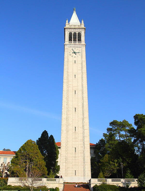
Choose one image of your own for Sections 1.1–1.5; the Campanile is only an example. Use the supplied preprocessing to center-crop and resize it to $512\times512$, with RGB values in $[-1,1]$. Sample one Gaussian noise tensor $\epsilon$ and reuse it to construct noisy images at $t\in\{0.25,0.50,0.75\}$. Larger $t$ retains more image information.

• Implement interpolate(image, noise, t).
• Show your original image and all three noisy images, labeled by time.

• torch.randn_like is useful for sampling $\epsilon$.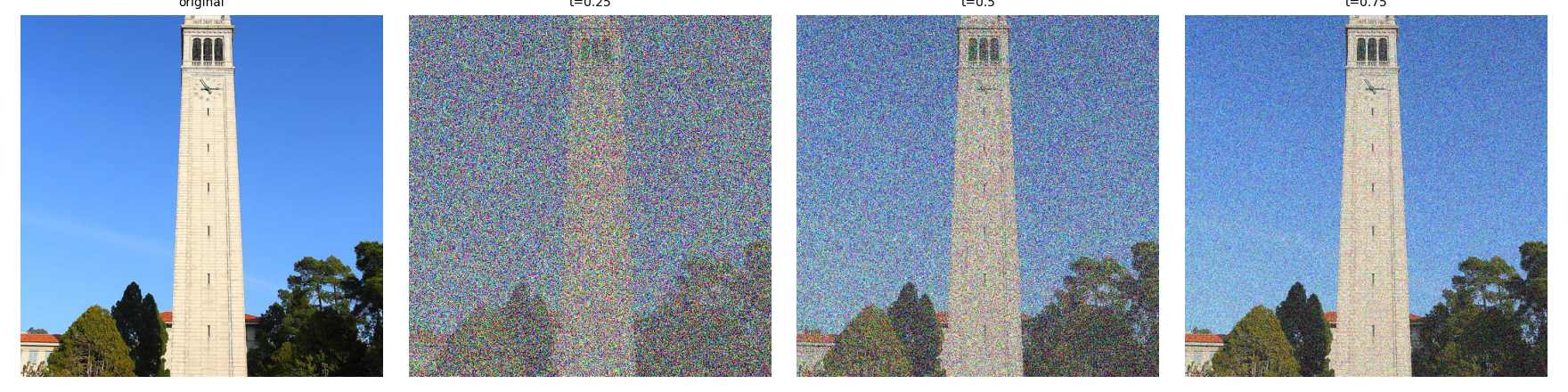
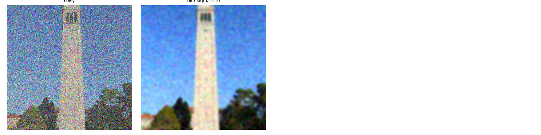
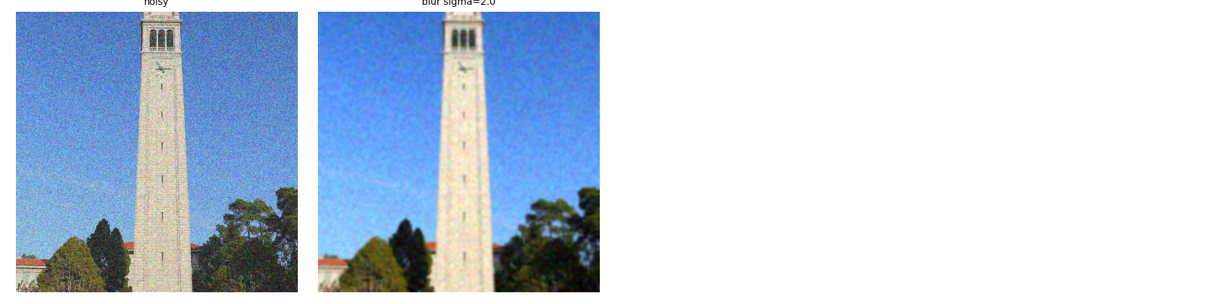
• Check both endpoints. Save the original image tensor, the sampled noise tensor, and all three noisy tensors for reuse in Sections 1.2–1.5. Section 1.4 needs the original image/noise pair to compute the ground-truth velocity.

Forward process

1.2 Classical Denoising

Use Gaussian blur as a baseline without a learned flow model. Averaging nearby pixels partially cancels independent, zero-mean noise. Stronger blur reduces noise but also removes image detail, so good results are difficult at high noise levels.

The image contribution in $x_t$ is scaled by $t$. For $t>0$, first restore its amplitude, then blur:

$$\frac{x_t}{t}=x_1+\frac{1-t}{t}\epsilon,\qquad \hat{x}_1^{\mathrm{blur}}=G_\sigma\!\left(\frac{x_t}{t}\right).$$

Here $G_\sigma$ is a Gaussian filter with standard deviation $\sigma$. Dividing by $t$ corrects the image amplitude; it does not remove noise. Apply this baseline to the saved inputs at $t=0.25,0.50,0.75$.

• For each of the three saved noisy versions of your own image from Section 1.1 ($t=0.25,0.50,0.75$), show the noisy input and your best Gaussian-denoised version side by side.

• torchvision.transforms.functional.gaussian_blur is useful. Here is the documentation.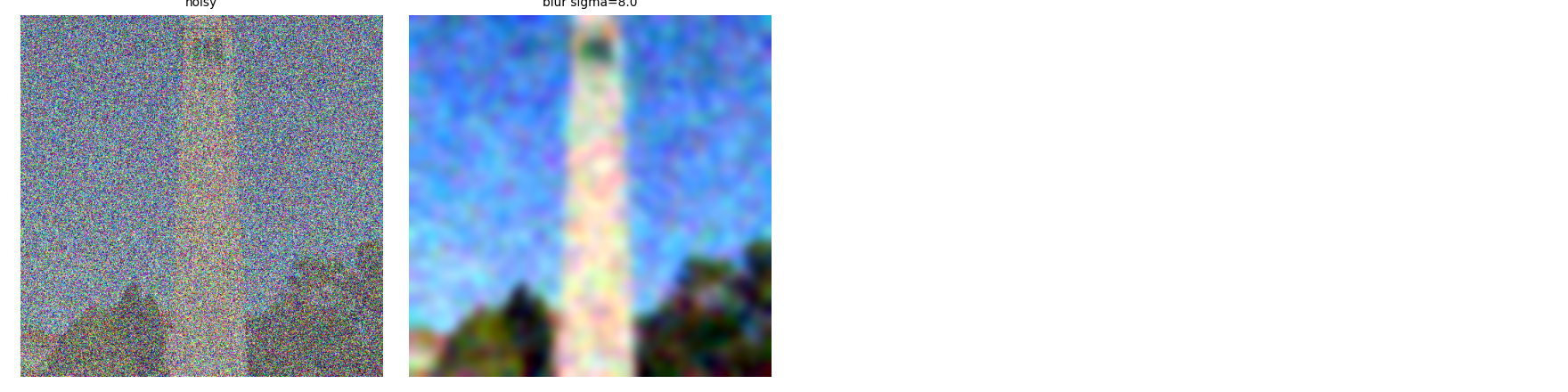

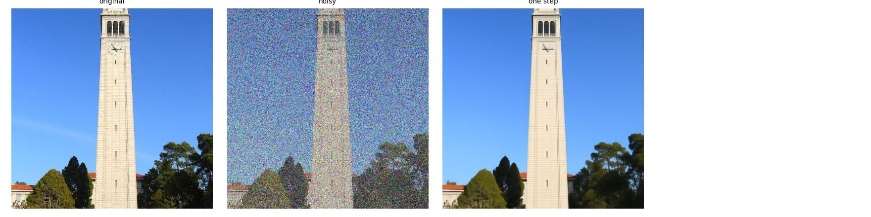
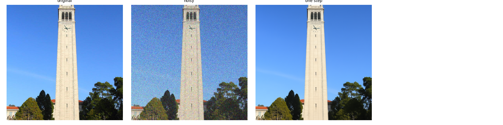
Gaussian blur comparison

1.3 One-Step Denoising

Now, we'll use a pretrained flow model to denoise. The supplied predict_velocity(x,t,condition) predicts the velocity at the noisy image and time. We can extrapolate to the clean endpoint using one prediction:

$$\hat{x}_1=x_t+(1-t)v_\theta(x_t,t,c).\tag{A.2}$$

Because this model was trained with text conditioning, we also need a text prompt embedding. Use the embedding for "a high quality photo". Later on, you can use your own text prompts.

• Implement one_step_denoise.
• For each of the three saved noisy versions of your own image at $t=0.25,0.50,0.75$, show the original, noisy input, and one-step estimate side by side.

• The prediction is velocity, not noise; use Equation A.2 rather than subtracting it.
• Check shape, dtype, and device: the adapter returns velocity with the same shape, dtype, and device as the input. Keep integration states float32; network evaluation is float32.
• Use torch.no_grad() when sampling to save memory. No gradients or model training are needed.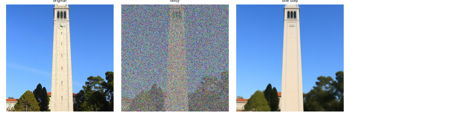

One-step denoising

1.4 Visualizing Velocity

In Section 1.3, we added $(1-t)\hat v_t$ to the noisy image to estimate the clean image. Here, we will visualize what the model adds.

Since we know the original image, we also know exactly what should be added: $x_1-x_t$. Compare this ground-truth update with the model's predicted update. An error heatmap shows where they differ most.

Use the same image of your own and saved noisy inputs from Section 1.1, at $t=0.25,0.50,0.75$, with the prompt "a high quality photo".

• Show the original image once.
• For each time $t=0.25,0.50,0.75$, display the noisy image $x_t$, predicted update $(1-t)\hat v_t$, ground-truth update $(1-t)v_{\mathrm{gt}}$, and an error heatmap, labeled by time.

• The predicted velocity is $\hat v_t=v_\theta(x_t,t,c)$. Using the saved noise from Section 1.1, the ground-truth velocity is $v_{\mathrm{gt}}=x_1-\epsilon$, so its update is $(1-t)v_{\mathrm{gt}}=x_1-x_t$.
• For the error heatmap, compute the root-mean-square (RMS) difference between the two updates across RGB at each pixel: $$E_t=\sqrt{\operatorname{mean}_{\mathrm{RGB}}\!\left(\big[(1-t)(\hat v_t-v_{\mathrm{gt}})\big]^2\right)}.$$ Square the channel differences, average over RGB, and take the square root. This gives one error value per pixel. Compute it before display scaling or clipping.
• Display all predicted and ground-truth updates on the same symmetric RGB scale, with zero at middle gray.
• Use matplotlib.pyplot.imshow with a linear color scale for the error maps. Choose vmin and vmax to make the errors visible, keeping the same limits across all three times.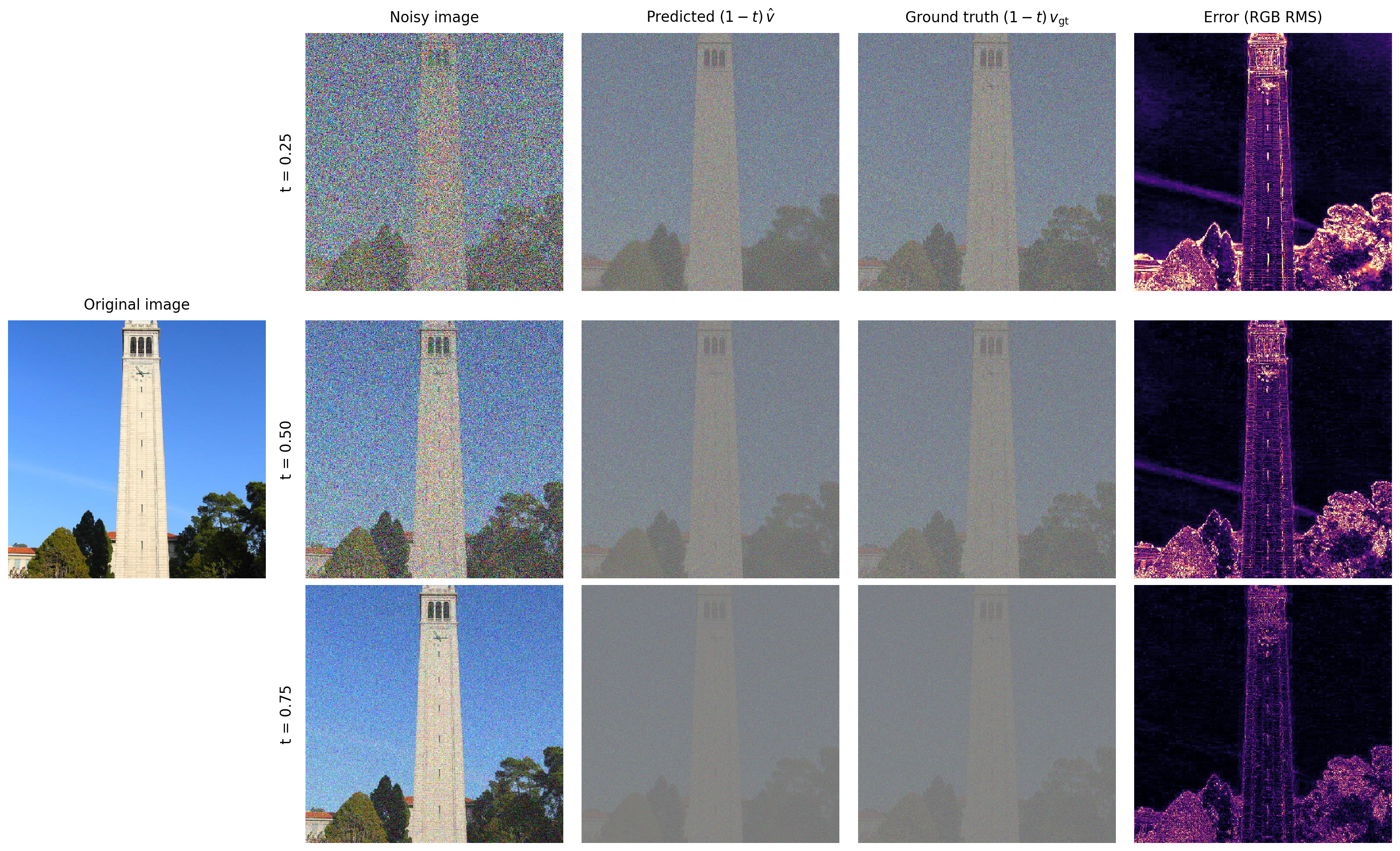

1.5 Iterative Denoising with Euler Sampling

One-step denoising can be inaccurate because the learned velocity changes as we move along the path. Instead, take a small step, predict a new velocity, and repeat. We use Euler integration:

$$x_{t+h}=x_t+h\,v_\theta(x_t,t,c).\tag{A.3}$$

Implement euler_sample(x_start,t_start,step_size,velocity). Use $h=0.02$ and shorten the last step if necessary to end exactly at $t=1$.

• Implement euler_sample. Starting with the saved $t=0.50$ noisy version of your own image, perform 25 Euler updates.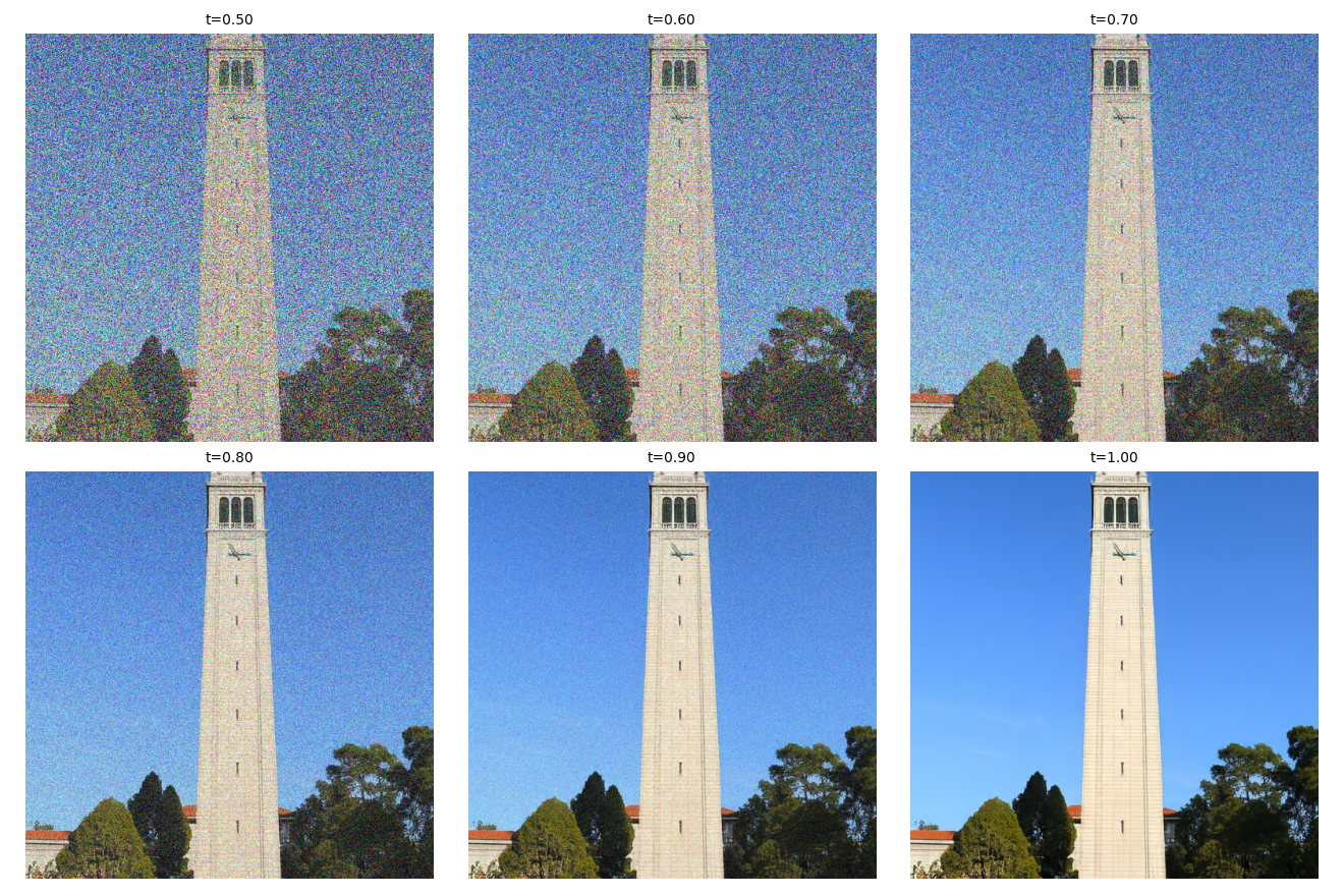
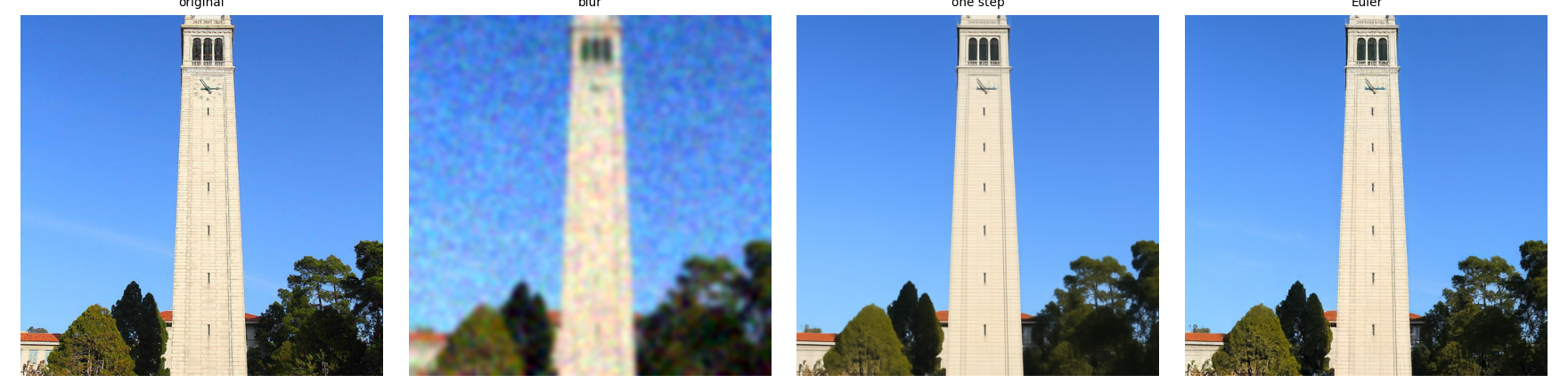
• Show the initial state, every fifth update, and final image, labeled by time.
• Compare the final result with your original image, one-step denoising (Section 1.3), and Gaussian blur (Section 1.2), using the same noisy input.

• Recompute velocity after each update. Return both the final image and saved states.
• Test a constant velocity field analytically, including a starting time that needs a shortened final step.

Euler denoising trajectory

Denoising methods

1.6 Generating Images from Noise

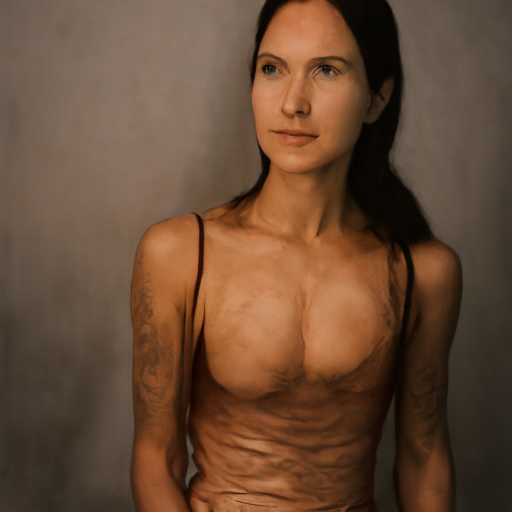
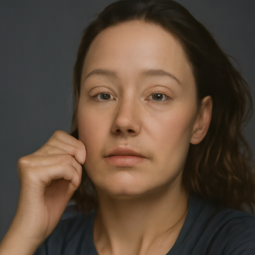
In Section 1.5, we use the flow model to denoise an image. Another thing we can do with the euler_sample function is to generate images from scratch. We can do this by setting t_start = 0 and passing x_start as random noise. This effectively denoises pure noise. Please do this, and show 5 results of the prompt"a high quality photo".

Deliverables

• Show 5 sampled images.

Hints

• Use torch.randn to make the noise.
• Make sure you move the tensor to the correct device and correct data type (float32) and use .to(device).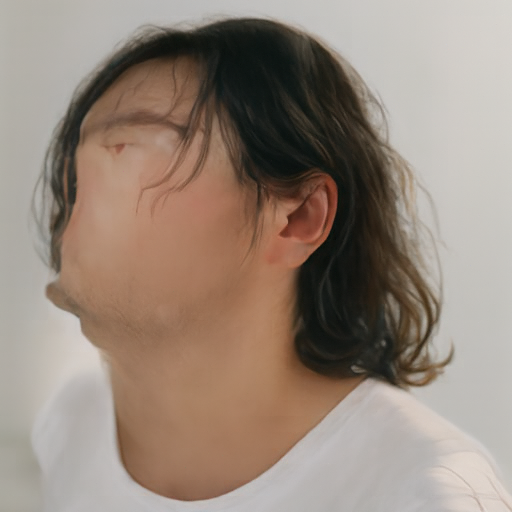
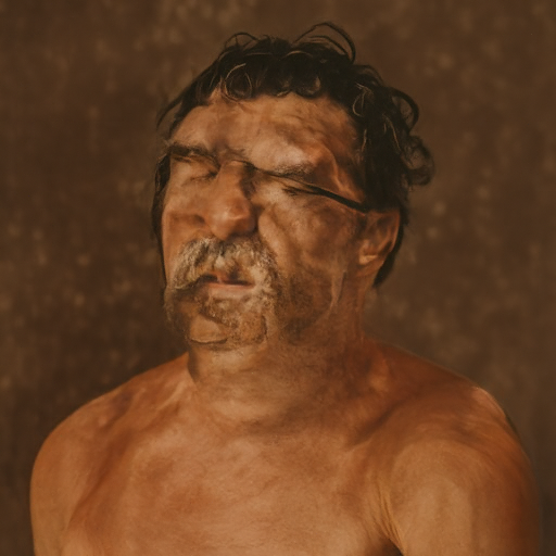
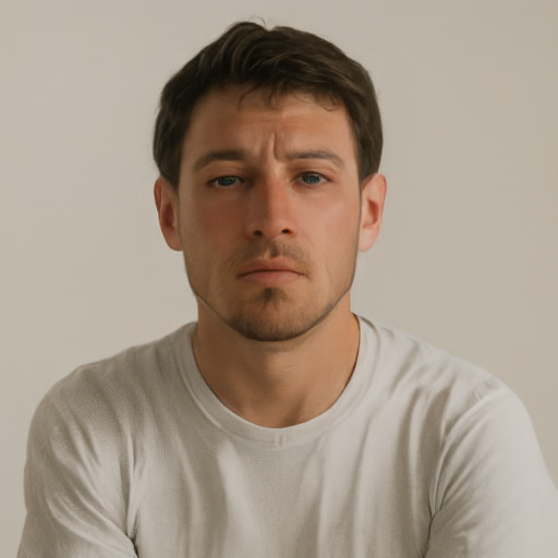
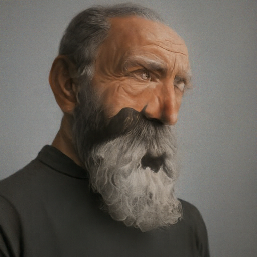
• The generic prompt may favor particular subjects; report what you observe. In Section 2, we will explore how CFG changes prompt alignment and diversity.

Conditional samples

2. Conditional Generation and Guidance

Conditional generation means generating an image given information such as a text prompt. Section 1 used a fixed prompt. Here you will strengthen the effect of that prompt using classifier-free guidance (CFG).

2.1 Classifier-Free Guidance (CFG)

You may have noticed that the generated images in the prior section are not very good. To improve prompt alignment and image quality, at the expense of diversity, we can use Classifier-Free Guidance (CFG).

Evaluate the same image and time with a conditional prompt and an empty-string prompt, obtaining $v_c$ and $v_u$. Combine them using:

$$v_{\mathrm{cfg}}=v_c+w(v_c-v_u).\tag{A.4}$$

Use $w=7$ and Euler step size $h=0.02$. Here $w=0$ is ordinary conditional sampling.

• Implement cfg_velocity.
• Show five CFG samples with "a high quality photo", using the same initial noises as Section 1.6. Compare the results.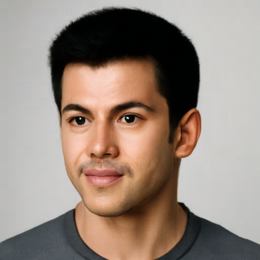

• Both predictions must use the same $x_t$ and $t$. Use the empty-string embedding for the unconditional branch.
• Check that $w=0$ reproduces the conditional prediction.

Classifier-free guidance

3. Creative Applications

Use flow sampling to edit existing images and generate optical illusions. Throughout this section, use Euler step size $h=0.02$, CFG weight $w=7$, and the empty prompt "" for the unconditional prediction.

3.1 Image-to-Image Editing

Download the Campanile image for Sections 3.1 and 3.2.

In Section 1.5, we take a real image, add noise to it, and then denoise. This effectively allows us to make edits to existing images. The more noise we add, the larger the edit will be. This works because in order to denoise an image, the flow model must to some extent "hallucinate" new things -- the model has to be "creative." Another way to think about it is that the denoising process "forces" a noisy image back onto the manifold of natural images.

Here, we're going to take the original Campanile image, noise it a little, and force it back onto the image manifold with the generic photo prompt. Effectively, we're going to get an image that is similar to the Campanile (with a low-enough noise level). This is inspired by the SDEdit algorithm.

To start, please run the forward process to get a noisy Campanile, and then run the edit function using a starting time of $[0.02,0.04,0.06,0.10,0.14,0.25,0.5]$ and show the results, labeled with the starting time. You should see a series of "edits" to the original image, gradually matching the original image closer and closer.

• Edits of the Campanile image, using the given prompt at starting times $[0.02,0.04,0.06,0.10,0.14,0.25,0.5]$ with the conditional text prompt "a high quality photo"
• Edits of 2 of your own test images, using the same procedure.

Hints

• You should have a range of images, gradually looking more like the original image

Campanile

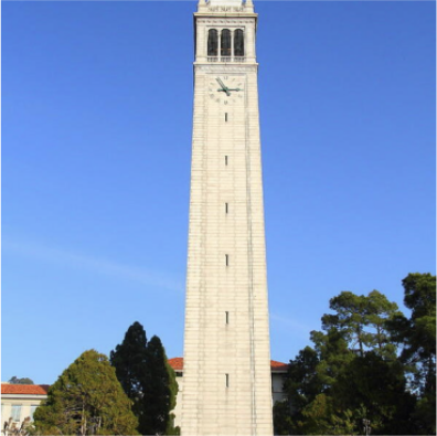
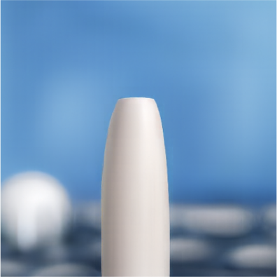
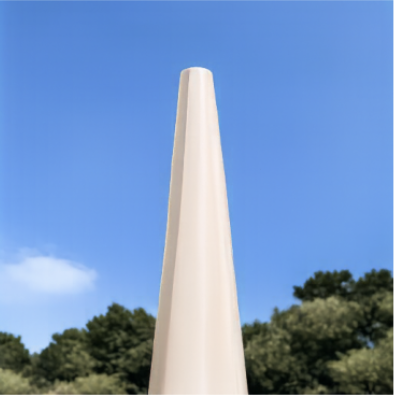
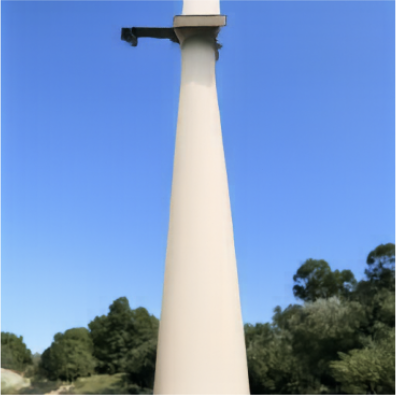
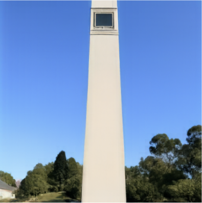
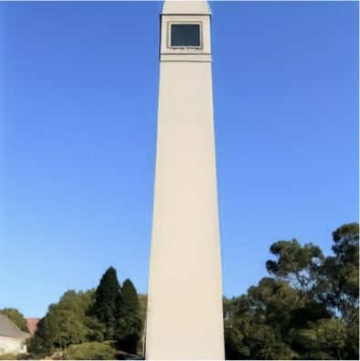
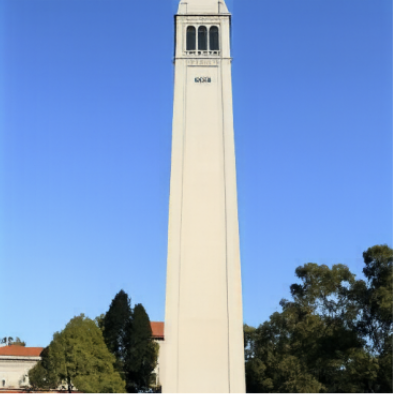
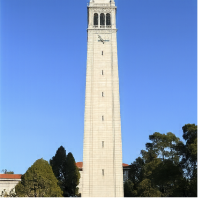
At $t=0.02$ only a pale vertical shape against blue survives. The tower sharpens as the starting time rises, but the clock face and belfry arches do not come back until $t=0.25$.

Pixel bear

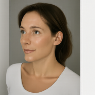
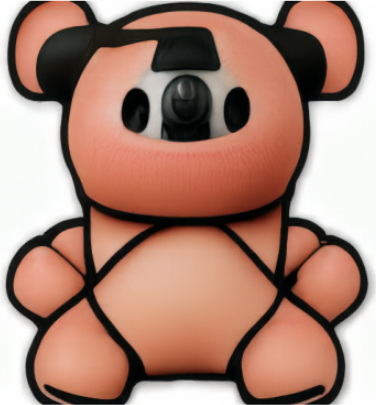
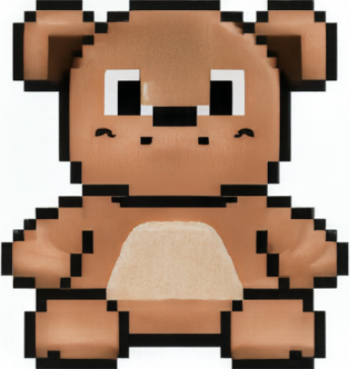
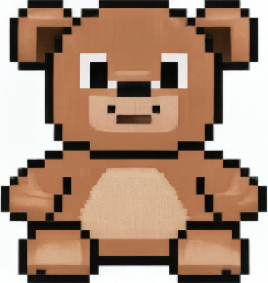
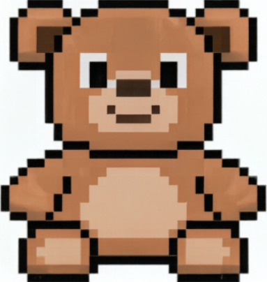
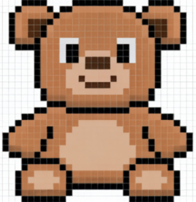
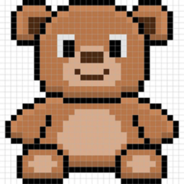
Starting times run from most noise (left) to least. At $t=0.02$ the input is gone entirely and the sampler generates an unrelated photo; by $t=0.25$ the pixel art returns almost unchanged.

Editing Hand-Drawn and Web Images

This procedure works particularly well if we start with a nonrealistic image (e.g. painting, a sketch, some scribbles) and project it onto the natural image manifold.

Please experiment by starting with hand-drawn or other non-realistic images and see how you can get them onto the natural image manifold in fun ways.

We provide you with 2 ways to provide inputs to the model:

1. Download images from the web
2. Draw your own images

Please find an image from the internet and apply edits exactly as above. And also draw your own images, and apply edits exactly as above. Feel free to copy the prior cell here. For drawing inspiration, you can check out the examples on this project page.

Deliverables

• 1 image from the web of your choice, edited using the above method for starting times $[0.02,0.04,0.06,0.10,0.14,0.25,0.5]$ (and whatever additional starting times you want)
• 2 hand drawn images, edited using the above method for starting times $[0.02,0.04,0.06,0.10,0.14,0.25,0.5]$ (and whatever additional starting times you want)

• We provide you with preprocessing code to convert web images to the format expected by PixNerd
• We need a square image. The supplied code center-crops and resizes to 512×512, so just draw in the middle of the canvas.

Web image

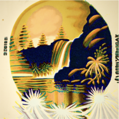
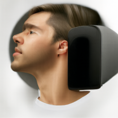
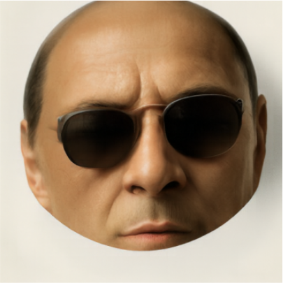
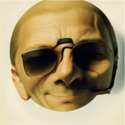
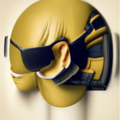
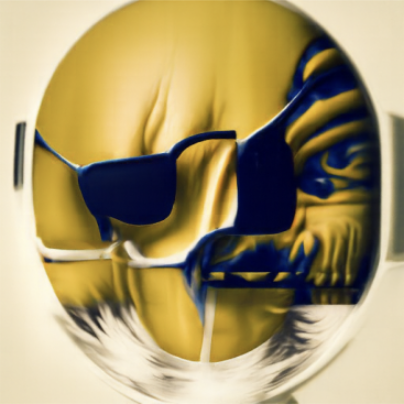
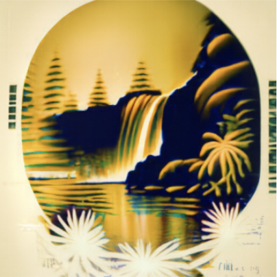
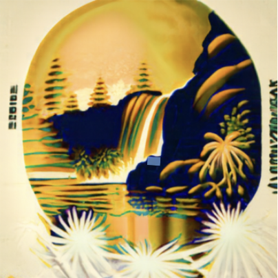
The same sweep on a downloaded image. Between $t=0.04$ and $t=0.14$ the sampler reads the oval frame and dark shapes as a face, and only the original's color palette survives; by $t=0.25$ the waterfall is back.

House drawing

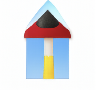
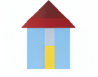
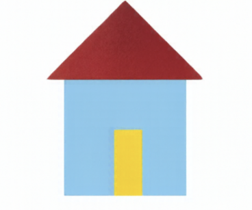
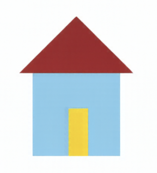
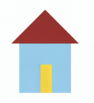
A flat drawing gives the sampler very little to hold on to: at $t=0.02$ it produces a portrait instead, and at $t=0.04$–$t=0.06$ it reads the roof and door as a figure under a peaked shape. The drawing returns by $t=0.10$.

Flower drawing

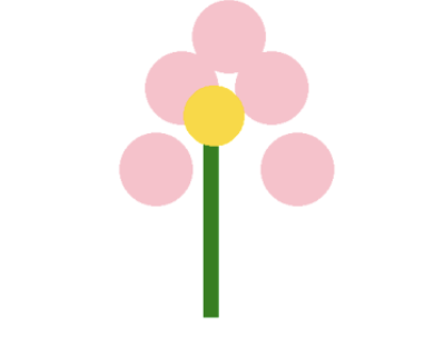
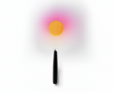
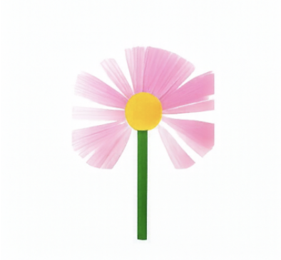
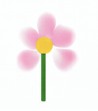
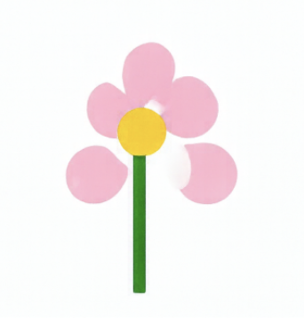
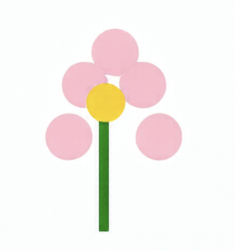
The low starting times keep only the round pink mass and the stem, reading them as an object on a stick. A recognizable flower appears at $t=0.10$, and by $t=0.25$ the petals are back to flat circles.

3.2 Text-Guided Image Editing

Use the same image-to-image editing procedure as Section 3.1, but replace "a high quality photo" with a prompt of your choice that describes the desired edit. The prompt guides how the model changes the image.

• Edits of the Campanile, using a prompt of your choice at starting times $[0.02,0.04,0.06,0.10,0.14,0.25,0.5]$. Show the prompt with your results.
• Edits of 2 of your own test images, using the same procedure and starting times. Choose a prompt for each image and show it with the results.

• Larger starting times preserve more of the original image. Smaller starting times add more noise and give the model more room to change the image according to the prompt.

Campanile → rocket ship

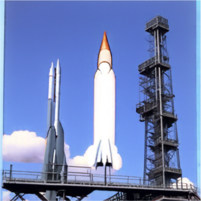
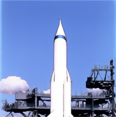
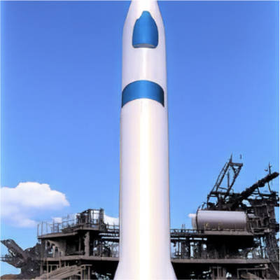
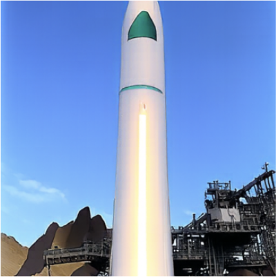
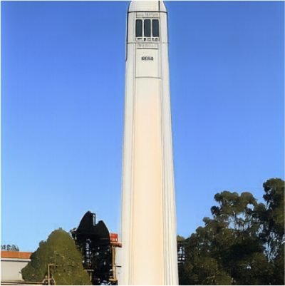
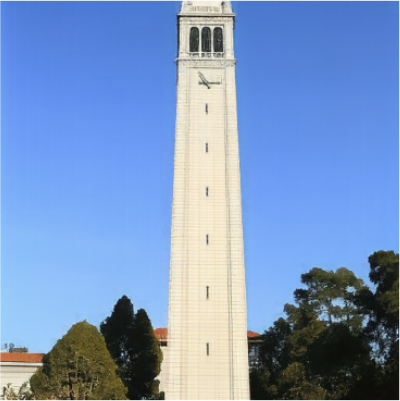
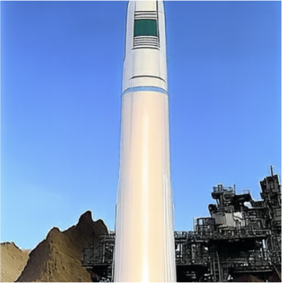
Prompt: "a photograph of a rocket on a launch pad". The prompt wins at the low starting times and the tower wins at the high ones; in between, at $t=0.06$–$t=0.14$, the result keeps the Campanile's framing and proportions while the surface becomes a rocket.

Text-guided bear editing

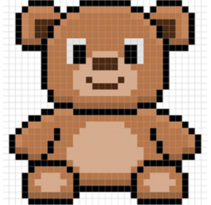
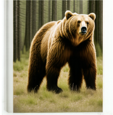
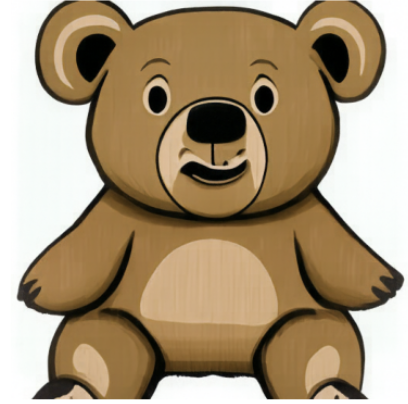
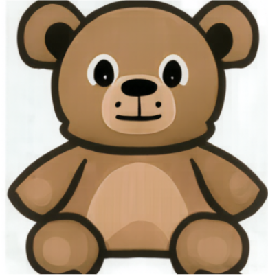
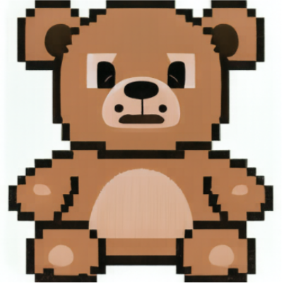
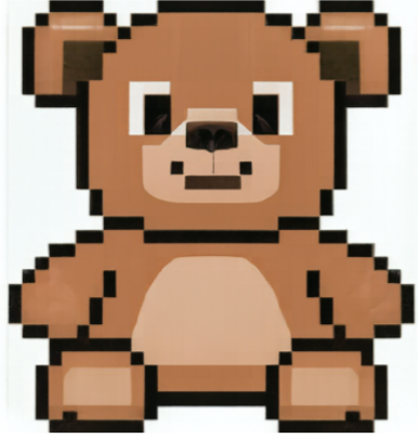
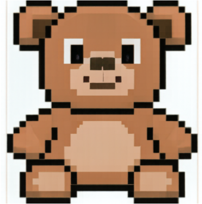
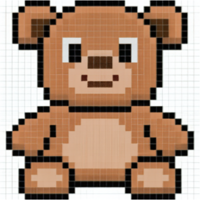
Prompt: "a photograph of a brown bear in a forest". Only $t=0.02$ reaches an actual photograph. At $t=0.04$–$t=0.06$ the prompt redraws the toy as a smoothly shaded illustration.

3.3 Visual Anagrams

In this part, we are finally ready to implement Visual Anagrams and create optical illusions with flow models. In this part, we will create an image that looks like "an oil painting of an old man", but when flipped upside down will reveal "an oil painting of people around a campfire".

To do this, we will denoise an image $x_t$ at step $t$ normally with the prompt $p_1$, to obtain velocity estimate $v_1$. But at the same time, we will flip $x_t$ upside down, and denoise with the prompt $p_2$, to get velocity estimate $v_2$. We can flip $v_2$ back, and average the two velocity estimates. We can then perform a Euler step with the averaged velocity estimate.

The full algorithm will be:

$$ v_1 = \text{CFG velocity}(x_t, t, p_1) $$

$$ v_2 = \text{flip}(\text{CFG velocity}(\text{flip}(x_t), t, p_2)) $$

$$ v = (v_1 + v_2) / 2 $$

where CFG velocity is the guided flow prediction from Section 2.1, $\text{flip}(\cdot)$ rotates the image by 180 degrees (flips both spatial axes, not just one), and $p_1$ and $p_2$ are two different text prompt embeddings. And our final velocity estimate is $v$. Please implement the above algorithm and show example of an illusion.

• Correctly implemented visual_anagrams function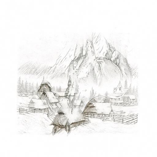
• 2 illusions of your choice that change appearance when you flip it upside down (feel free to take inspirations from this page).

• You may have to run multiple times to get a really good result for the same reasons as above.

Visual anagrams

3.4 Hybrid Images

In this part we'll adapt Factorized Diffusion and create hybrid images just like in project 2.

In order to create hybrid images with a flow model we can use a similar technique as above. We will create a composite velocity estimate $v$, by predicting velocity with two different text prompts, and then combining low frequencies from one velocity estimate with high frequencies of the other. The algorithm is:

$ v_1 = \text{CFG velocity}(x_t, t, p_1) $

$ v_2 = \text{CFG velocity}(x_t, t, p_2) $

$ v = f_\text{lowpass}(v_1) + f_\text{highpass}(v_2)$

where CFG velocity is the guided flow predictor, $f_\text{lowpass}$ is a low pass function, $f_\text{highpass}$ is a high pass function, and $p_1$ and $p_2$ are two different text prompt embeddings. Our final velocity estimate is $v$. Please show an example of a hybrid image using this technique (you may have to run multiple times to get a really good result for the same reasons as above). We recommend that you use a gaussian blur of kernel size 265 and sigma 16 at 512×512. Use the composite velocity in the Euler update. The high-pass component is the prediction minus its low-pass version.

• Correctly implemented make_hybrids function
• 2 hybrid images of your choosing (feel free to take inspirations from this page).

• use torchvision.transforms.functional.gaussian_blur
• You may have to run multiple times to get a really good result for the same reasons as above

Hybrid images — full size and distant views

Bells & Whistles

• More visual anagrams! Visual anagrams in Section 3.3 are created by flipping images upside down. However, there are much more transformations that also create visual anagrams! Refer to this paper and select two more transformations to create visual anagrams.
• Design a course logo! Doing text-conditioned image-to-image translation on UCB's logo or your drawing may be a good idea.

• Your own ideas: Be creative!

Deliverable Checklist

• Make sure that your website and submission include all the deliverables in each section above.
• Submit your PDF and code to corresponding assignments on Gradescope.
• The Google Form is not required for Part A; you only need to complete the Google Form after both parts are finished.

Acknowledgements

This project was a joint effort by Daniel Geng, Ryan Tabrizi, Hang Gao, Jingfeng Yang, Jameson Crate, Himanshu Gaurav Singh, Eric Khodorenko, and Kelvin Li, advised by Liyue Shen, Andrew Owens, and Alexei Efros.